In this blog post, we will show how to use the diffusers
library to upscale images using the Stable Diffusion Upscaler model. The model is a diffusion-based super-resolution model that is capable of generating high-quality upscaled images.
The diffusers
library provides a simple and easy-to-use interface for working with the Stable Diffusion Upscaler model. This blogpost will assume you have installed the diffusers
library and have access to a GPU. If you haven’t installed the library yet, follow the instructions to install the library in the official documentation. You can also take a look at my [blog post]/2023/09/16/How-I-Ran-Textual-Inversion.html, which covers how to set up the library on an AWS EC2 instance.
Let us get started with imports and setting up a pipeline to do the upscaling. The pipeline will take care of loading the models and weights and provide a simple interface that takes as input an image and returns the upscaled image.
from PIL import Image
import numpy as np
from diffusers import StableDiffusionUpscalePipeline
import torch
# load model and scheduler
model_id = "stabilityai/stable-diffusion-x4-upscaler"
pipeline = StableDiffusionUpscalePipeline.from_pretrained(
model_id, revision="fp16", torch_dtype=torch.float16,
)
pipeline = pipeline.to("cuda")
/home/ubuntu/fusion/lib/python3.8/site-packages/diffusers/pipelines/pipeline_utils.py:269: FutureWarning: You are loading the variant fp16 from stabilityai/stable-diffusion-x4-upscaler via `revision='fp16'` even though you can load it via `variant=`fp16`. Loading model variants via `revision='fp16'` is deprecated and will be removed in diffusers v1. Please use `variant='fp16'` instead.
warnings.warn(
text_encoder/model.safetensors not found
Loading pipeline components...: 100%|██████████| 6/6 [00:01<00:00, 5.41it/s]
/home/ubuntu/fusion/lib/python3.8/site-packages/diffusers/pipelines/stable_diffusion/pipeline_stable_diffusion_upscale.py:130: FutureWarning: The configuration file of the vae does not contain `scaling_factor` or it is set to 0.18215, which seems highly unlikely. If your checkpoint is a fine-tuned version of `stabilityai/stable-diffusion-x4-upscaler` you should change 'scaling_factor' to 0.08333 Please make sure to update the config accordingly, as not doing so might lead to incorrect results in future versions. If you have downloaded this checkpoint from the Hugging Face Hub, it would be very nice if you could open a Pull Request for the `vae/config.json` file
deprecate("wrong scaling_factor", "1.0.0", deprecation_message, standard_warn=False)
Let us download an image of a sunflower head and use it as an example for super-resolution. The image contains a lot of texture and detail, which makes it a good candidate to demonstrate the capabilities of the Stable Diffusion model for super-resolution.
!wget https://upload.wikimedia.org/wikipedia/commons/4/44/Helianthus_whorl.jpg
--2024-02-01 23:40:22-- https://upload.wikimedia.org/wikipedia/commons/4/44/Helianthus_whorl.jpg
Resolving upload.wikimedia.org (upload.wikimedia.org)... 198.35.26.112, 2620:0:863:ed1a::2:b
Connecting to upload.wikimedia.org (upload.wikimedia.org)|198.35.26.112|:443... connected.
HTTP request sent, awaiting response... 200 OK
Length: 327296 (320K) [image/jpeg]
Saving to: ‘Helianthus_whorl.jpg’
Helianthus_whorl.jp 100%[===================>] 319.62K --.-KB/s in 0.02s
2024-02-01 23:40:22 (19.4 MB/s) - ‘Helianthus_whorl.jpg’ saved [327296/327296]
img = Image.open('Helianthus_whorl.jpg')
img.size
(640, 480)
The model upscales to 4x the initial size (hence stable-diffusion-x4-upscale
) so let us downscale the image to a quarter of the original dimensions and then rescale using the model.
new_size = tuple(np.floor_divide(img.size, 4).astype('int'))
low_res_img = img.resize(new_size)
low_res_img.size
(160, 120)
We can see that the downscaled image is quite blurry with a lot of the textural details lost.
import matplotlib.pyplot as plt
import numpy as np
# List of image arrays
image_arrays = [img, low_res_img]
titles = ["Original Image", "Downscaled Image" ]
# Create subplots
fig, axes = plt.subplots(1, len(image_arrays), figsize=(15, 5))
# Iterate over image arrays and titles
for i, (img_array, title) in enumerate(zip(image_arrays, titles)):
axes[i].imshow(img_array)
axes[i].set_title(title)
axes[i].axis('off')
# Adjust layout and display the plot
plt.tight_layout()
Image credit: L. Shyamal, CC BY-SA 2.5 https://creativecommons.org/licenses/by-sa/2.5, via Wikimedia Commons
Upscaling using the super-resolution model is a simple matter of calling pipeline
with the prompt and image. There are other settings that can be adjusted such as the number of iterations and the number of images to generate. Refer to the documentation for more details. Here we will use the default settings of a single image and 75 iterations.
line = pipeline(prompt = 'Sunflower head displaying the floret arrangement',
image= low_res_img)
upscaled_image = line.images[0]
100%|██████████| 75/75 [00:13<00:00, 5.42it/s]
Since this model increases the size of the image by 4x and the input was the original image downscaled by 4x, the super-resolved image should be the same size as the original image.
upscaled_image.size
(640, 480)
Below we plot the downscaled input image, the downscaled image resized using bicubic interpolation, the super-resolution model output and the original image.
import matplotlib.pyplot as plt
# List of image arrays
image_arrays = [low_res_img, low_res_img.resize(img.size), upscaled_image, img]
titles = ["Downscaled", "Bicubic interpolation", "Super-resolution", "Original"]
# Create subplots
fig, axes = plt.subplots(2, 2, figsize=(15, 15))
axes = axes.ravel()
# Iterate over image arrays and titles
for i, (img_array, title) in enumerate(zip(image_arrays, titles)):
axes[i].imshow(img_array)
axes[i].set_title(title, fontsize=16)
axes[i].axis('off')
# Adjust layout and display the plot
plt.tight_layout()
Image credit: L. Shyamal, CC BY-SA 2.5 https://creativecommons.org/licenses/by-sa/2.5, via Wikimedia Commons
It can be seen that the super-resolved image is superior to the one rescaled using bicubic interpolation and restores a lot of the textural detail that had gotten lost during downscaling. However it is not perfect. For example, the innermost florets have the same shape as the outer ones, whereas in the original image they are pointy and directed inwards. This area in the downscaled image is quite blurred and the model fails to recover the details of the original image.
In this simple example, we have only touched on the basics of diffusion-based super-resolution and the capabilities of the Stable Diffusion Upscaler model in order to get you started. I encourage you to explore the various settings and options that can be adjusted to obtain different and possibly better results.
]]>This blog post will guide you through the steps of creating matrices in LaTeX. It will start with the general syntax and then explain how to create row and column vectors, determinants, arbitrary sized matrices and nested matrices. It will conclude with several examples of real world matrices and the use of matrices in mathematical expressions.
In LaTeX, matrices are created using the “bmatrix” environment. The general syntax for a matrix is as follows:
\begin{bmatrix}
a & b & c \\
d & e & f \\
g & h & i \\
\end{bmatrix}
Replace the placeholders (a, b, c, etc.) with your desired matrix elements. The ampersand (&
) is used to separate columns, and the double backslash (\\
) indicates the end of a row.
Both column and row vectors are essentially specialized forms of matrices, and you can use the “bmatrix” environment to represent them.
To create a column vector, you can use the “bmatrix” environment with a single column:
\begin{bmatrix}
a \\
b \\
c \\
\end{bmatrix}
Similarly, a row vector is a matrix with a single row:
\begin{bmatrix}
a & b & c
\end{bmatrix}
LaTeX supports various bracket types for matrices.
To represent matrices with parentheses $(\cdot)$ you can use the “pmatrix” environment:
\begin{pmatrix}
a & b \\
c & d \\
\end{pmatrix}
To represent determinants, you can use the “vmatrix” or “Vmatrix” environments:
vmatrix: Vertical bars $\vert \cdot \vert$ as brackets
\begin{vmatrix}
a & b \\
c & d \\
\end{vmatrix}
Vmatrix: Double vertical $\Vert \cdot \Vert$ bars as brackets
\begin{Vmatrix}
a & b \\
c & d \\
\end{Vmatrix}
To structure data in a matrix format without any brackets, you can use the “matrix” environment:
\begin{matrix}
a & b \\
c & d \\
\end{matrix}
Sometimes you want to represent a range of elements in a matrix without explicitly listing them all. For example when you have an arbitrary $m \times n$ matrix and you want to show only a few representative elements.
For this, you can use ellipses. There are different commands for horizontal, vertical and diagonal ellipses
The \dots
(or \ldots
) command can be used to represent a range of skipped elements in a row. For example, here is row vector showing only the first two and last of $n$ elements
\begin{bmatrix}
a_1 & a_2 & \dots & a_n
\end{bmatrix}
The \vdots
command can be used to represent a range of skipped elements in a column. For example, here is column vector showing only the first two and last of $n$ elements
\begin{bmatrix}
a_1 \\
a_2 \\
\ldots \\
a_n
\end{bmatrix}
The \ddots
command, often used in combination with \dots
and \vdots
can be used to skip columns and rows simultaneously.
\begin{bmatrix}
a_{11} & \dots & a_{1n} \\
\vdots & \ddots & \vdots \\
a_{n1} & \dots & a_{nn} \\
\end{bmatrix}
Matrix elements can be arbitrary LaTeX expressions and the matrix will automatically adjust to accommodate the size of the expression.
R = \begin{bmatrix}
\cos \theta &-\sin \theta \\
\sin \theta &\cos \theta
\end{bmatrix}
\nabla \times \mathbf {F} =
\begin{vmatrix}
\boldsymbol {\hat {\imath }} & {\boldsymbol {\hat {\jmath }}} & {\boldsymbol {\hat {k}}}
\\ frac {\partial }{\partial x} & \frac {\partial }{\partial y} & \frac {\partial }{\partial z}\\F_{x} & F_{y} & F_{z}
\end{vmatrix}
W = \frac{1}{\sqrt{N}} \begin{bmatrix}
1 & 1 & 1 & 1 & \cdots & 1 \\
1 & \omega & \omega^2 & \omega^3 & \cdots & \omega^{N-1} \\
1 & \omega^2 & \omega^4 & \omega^6 & \cdots & \omega^{2(N-1)} \\
1 & \omega^3 & \omega^6 & \omega^9 & \cdots & \omega^{3(N-1)} \\
\vdots & \vdots & \vdots & \vdots & \ddots & \vdots \\
1 & \omega^{N-1} & \omega^{2(N-1)} & \omega^{3(N-1)} & \cdots & \omega^{(N-1)(N-1)}
\end{bmatrix}
where $\omega = e^{-2\pi i/N}$
You can also nest matrices within matrices. Here’s an example of a block diagonal matrix that represents an important quantum computing logic gate called the CNOT gate:
\begin{bmatrix}
I_2 & 0 \\
0 & X
\end{bmatrix}
= \begin{bmatrix}
\begin{bmatrix}
1 & 0 \\
0 & 1
\end{bmatrix} & 0 \\
0 & \begin{bmatrix}
0 & 1 \\
1 & 0
\end{bmatrix}
\end{bmatrix}
where $I_2$ is the $2 \times 2$ identity matrix and $X$ is the Pauli-X matrix
You can nest matrices to any depth as needed. For example, the matrix for another quantum logic gate, the Toffoli gate is a block diagonal matrix with a nested matrix in the bottom right corner:
\begin{bmatrix}
I_4 & 0 \\
0 & CNOT
\end{bmatrix}
= \begin{bmatrix}
I_4 & 0 \\
0 & \begin{bmatrix}
I_2 & 0 \\
0 & X
\end{bmatrix}
\end{bmatrix}
= \begin{bmatrix}
I_4 & 0 \\
0 & \begin{bmatrix}
\begin{bmatrix}
1 & 0 \\
0 & 1
\end{bmatrix} & 0 \\
0 & \begin{bmatrix}
0 & 1 \\
1 & 0
\end{bmatrix}
\end{bmatrix}
\end{bmatrix}
where $I_4$ is the $4 \times 4$ identity matrix.
Matrices can be incorporated into mathematical expressions just like any other variable. For example, here of the rotation of an arbitrary vector $\mathbf{v}$ by an angle $\theta$:
R\mathbf {v} =
\begin{bmatrix}
\cos \theta &-\sin \theta \\
\sin \theta &\cos \theta
\end{bmatrix}
\begin{bmatrix}
x\\y
\end{bmatrix}=
\begin{bmatrix}
x\cos \theta -y\sin \theta
\\x\sin \theta +y\cos \theta
\end{bmatrix}
Here is another example of the exponential of a diagonal matrix that demonstrates how matrices in LaTeX can be seamlessly integrated into a variety of mathematical expressions and how they play nicely with other LaTeX capabilities like superscripts and brackets.
\begin{aligned}
e^{\operatorname{diag}\left(
\begin{bmatrix}
a_1 \\
a_2
\end{bmatrix}
\right)} &= \exp\left(\begin{bmatrix}
a_1 & 0 \\
0 & a_2
\end{bmatrix}\right)
\\&= \sum_{i=0}^\infty \frac{1}{i!} \begin{bmatrix}
a_1 & 0 \\
0 & a_2
\end{bmatrix}^i
\\&= \sum_{i=0}^\infty \frac{1}{i!} \begin{bmatrix}
a_1^i & 0 \\
0 & a_2^i
\end{bmatrix}
\\&= \begin{bmatrix}
e^{a_1} & 0 \\
0 & e^{a_2}
\end{bmatrix}
\end{aligned}
In this blog post we covered the key features of representing matrices in LaTeX. You should now be able to create a variety of matrices and incorporate them in your LaTeX code.
Quantum computing is a rapidly growing field that leverages the principles of quantum mechanics to process information. One of the pillars of quantum computing is the quantum circuit, a model for quantum computation in which a computation is represented by a sequence of quantum gates. In this blog we will learn how to create quantum gate and quantum circuit diagrams in Python using the SymPy library.
SymPy is a Python library for symbolic mathematics. It includes a module for quantum computing called sympy.physics.quantum
which we will use to create quantum gates and circuits and to generate their diagrams. We will start from simple single qubit gates to more complex two qubit gates and finally learn to create custom gates and quantum circuits.
This tutorial assumes that you have basic knowledge of quantum computing and quantum gates. I am planning on writing a blog on quantum gates soon, but until then I recommend this Wikipedia article as a good reference for quantum gates.
Let’s start by creating an X gate, also known as a NOT gate. The X gate acts on a single qubit. It is represented by the following matrix:
\[X = \begin{bmatrix}0 & 1 \\ 1 & 0\end{bmatrix}\]SymPy has a number of commonly used quantum gates already defined. To instantiate a gate, you need to specify the qubit or qubits it acts.
Key qubit numbering conventions in SymPy:
Let’s now create an X gate acting on the first qubit.
from sympy.physics.quantum.gate import X
gate = X(0)
In order to plot our quantum gate, we’ll use the plot
function from the circuitplot
module. The plot
function takes two arguments, the gate and the number of qubits in the circuit. Let’s plot the X gate we created above.
import sympy.physics.quantum.circuitplot as plot
plot.circuit_plot(gate, 1);
Saving the generated quantum circuit figure is a straightforward process. You can use the savefig
function from the matplotlib
package to save the figure. Let’s save the figure we generated above.
import matplotlib.pyplot as plt
plt.savefig("X_gate.png");
<Figure size 432x288 with 0 Axes>
The Hadamard gate or $H$ gate is a one-qubit gate which performs a Hadamard transform on the given qubit.
It is represented by the following matrix:
The steps to create a Hadamard gate are the same as the X gate. Let’s create a Hadamard gate acting on the first qubit and plot it.
from sympy.physics.quantum.gate import H
H_gate = H(0)
plot.circuit_plot(H_gate, 1);
Controlled NOT gate, or CNOT, is a two-qubit gate which takes two inputs, a control and a target qubit and applies a NOT to the target only when the control is $\left\vert 1\right>$. We use the notation CNOTxy to denote a gate where the qubit with index $x$ is the control and qubit with index $y$ is the target.
The matrix representation of CNOT21 i.e. CNOT with the second qubit as the control and the first qubit as the target is:
\[\begin{bmatrix} 1 & 0 & 0 & 0 \\ 0 & 1 & 0 & 0 \\ 0 & 0 & 0 & 1 \\ 0 & 0 & 1 & 0 \end{bmatrix}\]I should note that you may find other sources that represent the CNOT gate with the target qubit as the first qubit and the control qubit as the second qubit in which case the above would be the matrix representation of CNOT12. However I have tried to use notation that is consistent the way the gates are instantiated in SymPy.
The CNOT
class in SymPy takes two arguments, the control qubit index and the target qubit index in that order. Let us first construct and plot a CNOT21 gate.
from sympy.physics.quantum.gate import CNOT
CNOT_21 = CNOT(1, 0) # Note the zero based indexing so that 2->1, 1->0
plot.circuit_plot(CNOT_21, 2);
Note that in the diagram the the qubits are numbered from top to bottom. The topmost wire corresponds the first index, the second wire to the second index and so on. Now let’s plot a CNOT12 gate, where the control and the target are reversed.
CNOT_12 = CNOT(0, 1)
plot.circuit_plot(CNOT_12, 2);
If you look at the matrix for $X$ you can see that it flips qubits turning $\left\vert 0\right>$ to $\left\vert 1\right>$ and $\left\vert 1\right>$ to $\left\vert 0\right>$. (Recall that the vector representations of the qubits are $\left\vert 0\right> = [1, 0]^T$ and $\left\vert 1\right> = [0, 1]^T$).
The gate is often represented using the symbol $\oplus$ that’s used in the CNOT gate. X
has a built in function plot_gate_plus
that can plot the gate using this symbol but it is not used by circuit_plot
. Let us subclass X
to create XNOT
, where we redefine the plot_gate
function as an alias for the plot_gate_plus
function, maintaining identical functionality otherwise so that now circuit_plot
will plot X
using the desired symbol.
class XNOT(X):
plot_gate = X.plot_gate_plus
plot.circuit_plot(XNOT(0), 1);
You can use the UGate
class to create a custom quantum gate. As an example, we’ll create a rotation gate. The rotation of a qubit by an angle $\theta$ around the Y-axis of the Bloch sphere is represented by the following matrix:
Here, $R_Y(\theta)$ represents the Y-axis rotation gate, $I$ is the identity matrix, and $Y$ is the Pauli $Y$ matrix, which is defined as:
\[Y = \begin{bmatrix} 0 & -i \\ i & 0 \end{bmatrix}\]To create a Y rotation gate from the UGate class, you need to instantiate the class with the following arguments:
Let us write a simple function to create a Y rotation gate.
from sympy.physics.quantum.gate import UGate
import sympy as sy
def R_Y(qubit, theta):
Y_sy = sy.Matrix([[0, -sy.I], [sy.I, 0]])
gate = UGate(qubit, sy.eye(2)*sy.cos(theta/2) - sy.I * Y_sy * sy.sin(theta/2))
return gate
Let us now define an $R_Y\left(\frac{\pi}{4}\right)$ gate.
R_Y_piby4 = R_Y(0, sy.pi/4)
If you now try to plot the gate, this is what it looks like:
plot.circuit_plot(R_Y_piby4, 1);
As you can see this is labeled as a generic $U$ gate. To customize the label, you can modify the gate_name_latex
attribute of the gate. Let’s update the function accordingly.
def R_Y(qubit, theta):
Y_sy = sy.Matrix([[0, -sy.I], [sy.I, 0]])
gate = UGate(qubit, sy.eye(2)*sy.cos(theta/2) - sy.I * Y_sy * sy.sin(theta/2))
name = f'R_Y\\left({sy.latex(theta)}\\right)'
gate.gate_name_latex = name
gate.gate_name = name
return gate
Now, if you create and plot the gate again, you’ll see it is correctly labeled as $R_Y\left(\frac{\pi}{4}\right)$.
R_Y_piby4 = R_Y(0, sy.pi/4)
plot.circuit_plot(R_Y_piby4, 1);
We can also construct custom multi-qubit gates. As an example, let’s create a Toffoli gate which takes three inputs, two of which are controls whilst the other is the target. The Toffoli gate applies a NOT to target only when both controls are $\left\vert 1\right>$. It is effectively a controlled-CNOT gate.
The matrix representation of the Toffoli gate is:
\[\begin{bmatrix} 1 & 0 & 0 & 0 & 0 & 0 & 0 & 0 \\ 0 & 1 & 0 & 0 & 0 & 0 & 0 & 0 \\ 0 & 0 & 1 & 0 & 0 & 0 & 0 & 0 \\ 0 & 0 & 0 & 1 & 0 & 0 & 0 & 0 \\ 0 & 0 & 0 & 0 & 1 & 0 & 0 & 0 \\ 0 & 0 & 0 & 0 & 0 & 1 & 0 & 0 \\ 0 & 0 & 0 & 0 & 0 & 0 & 0 & 1 \\ 0 & 0 & 0 & 0 & 0 & 0 & 1 & 0 \end{bmatrix}\]To construct the Toffoli we can use the CGate
class. The CGate
class takes two arguments:
Since the Toffoli gate can be represented as controlled CNOT gate, we can create a Toffoli gate as follows:
from sympy.physics.quantum.gate import CGate
control_qubit1 = 2
control_qubit2 = 1
target_qubit = 0
toffoli_1 = CGate([control_qubit1], CNOT(control_qubit2, target_qubit))
plot.circuit_plot(toffoli_1, 3);
You can also regard the Toffoli gate as a doubly-controlled NOT gate where the first two qubits are controls and the third qubit is the target. In this case, we can create a Toffoli gate (using XNOT
to ensure the NOT symbol is used in the plot) as follows:
toffoli_2 = CGate([control_qubit1, control_qubit2], XNOT(target_qubit))
plot.circuit_plot(toffoli_2, 3);
As you can see, both the representations are equivalent and lead to identical gate diagrams.
A sequence of quantum gates gives rise to a quantum circuit. You can construct a quantum circuit in SymPy by multiplying gates together in the order in which you want them to be applied in the circuit
A simple quantum circuit uses $X$ and rotation gates to create a $H$ gate. It is straightforward to show that
\[H = R_Y\left(-\frac{\pi}{4}\right)X R_Y\left(\frac{\pi}{4}\right)\]Let’s create and plot the circuit in SymPy
circuit = R_Y(0, -sy.pi/4) * X(0) * R_Y(0, sy.pi/4)
plot.circuit_plot(circuit, 1);
Note that since the gates in the circuit are applied from left to right, the order of the gates in the circuit is the reverse of the order in which they are multiplied to form $H$. To confirm that the circuit is indeed equivalent to the $H$ gate, we can use the represent
function from the represent
module to get the matrix representation of the circuit.
from sympy.physics.quantum.represent import represent
represent(circuit, nqubits=1).simplify()
$\displaystyle \left[\begin{matrix}\frac{\sqrt{2}}{2} & \frac{\sqrt{2}}{2}\\frac{\sqrt{2}}{2} & - \frac{\sqrt{2}}{2}\end{matrix}\right]$
which is indeed the matrix representation of the Hadamard gate.
Now we will implement a more complex circuit involving 2 qubits. The CNOT has a certain property that if you apply a Hadamard gate to both qubits at the input as well as the output, you get a CNOT gate with the control and target qubits swapped.
Let’s see how this comes about. First, a Hadamard gate applied in parallel to both qubits gives rise to the following matrix
\[H\otimes H = \frac{1}{2}\begin{bmatrix} 1 & 1 & 1 & 1 \\ 1 & -1 & 1 & -1 \\ 1 & 1 & -1 & -1 \\ 1 & -1 & -1 & 1 \end{bmatrix}\]The CNOT12 gate has the following matrix
\[CNOT_{12} = \begin{bmatrix} 1 & 0 & 0 & 0 \\ 0 & 0 & 0 & 1 \\ 0 & 0 & 1 & 0 \\ 0 & 1 & 0 & 0 \end{bmatrix}\]Use these two matrices it is straightforward to show that
\[H\otimes H\cdot CNOT_{21}\cdot H\otimes H = CNOT_{12}\]Let us plot the circuit
circuit = H(0) * H(1) * CNOT_21 * H(0) * H(1)
plot.circuit_plot(circuit, 2);
We can also get the matrix representation of the circuit to confirm that it is indeed a CNOT12 gate.
matrix = represent(circuit, nqubits=2)
from IPython.display import Markdown
## Needed to make the matrix display correctly in the markdown document
Markdown(f'$${sy.latex(matrix)}$$')
In this blog, we learned how to create quantum gate and quantum circuit diagrams using Python’s SymPy library. We started by creating single qubit gates like the X gate and Hadamard gate. We then moved on to creating multi-qubit gates like the CNOT gate and Toffoli gate. Finally, we learned how to create custom gates and quantum circuits.
This only scratches the surface of SymPy’s quantum computing capabilities and of quantum computing in general. If you want to learn more about quantum computing, I recommend checking out the MIT Open Learning courses on Quantum Information Science (courses 8.370 and 8.371). For more about SymPy’s quantum computing capabilities, check out the SymPy documentation.
]]>In this blog post, we will explore how to implement a minimalist ChatGPT-style app in a Jupyter Notebook or command line. The goal is to provide an understanding of the important concepts, components, and techniques required to create a chat app on top of a large language model (LLM), specifically OpenAI’s GPT. The resulting chat app can serve as a foundation for creating your own customised conversational AI applications.
The code in this blog post can be found in a notebook here. The script for the command line version can be found here.
Let us begin with a quick overview of the Chat Completions endpoint of the OpenAI API, which enables you to interact with OpenAI’s large language models to generate text-based responses in a conversational manner. It’s designed for both single-turn tasks and multi-turn conversations.
Example API Call:
The provided code snippet demonstrates how to make an API call for chat completions. In this example, the chat model used is “gpt-3.5-turbo,” and a conversation is created with system, user, and assistant messages:
response = openai.ChatCompletion.create(
model="gpt-3.5-turbo",
messages=[
{"role": "system", "content": "You are a helpful assistant."},
{"role": "user", "content": "Who wrote 'A Tale of Two Cities'?"},
{"role": "assistant", "content": "Charles Dickens wrote 'A Tale of Two Cities'."},
{"role": "user", "content": "When was it first published?"}
]
)
Message Structure:
messages
parameter, which is an array of message objects.role
(either “system,” “user,” or “assistant”) and content
(the text of the message).Typical Conversation Format:
A typical conversation format starts with a system message, followed by alternating user and assistant messages. The system message helps set the behavior of the assistant, but it’s optional. If omitted, the model’s behavior will be similar to a generic message like “You are a helpful assistant.”
Importance of Conversation History:
Including conversation history is crucial when user instructions refer to prior messages. The model has no memory of past requests, so all relevant information must be supplied within the conversation history. If a conversation exceeds the model’s token limit, it needs to be shortened.
Now let write a set of functions for communicating with OpenAI’s Chat Completions API. These functions will serve as the backbone of our minimalist chat app. Each function plays a specific role in managing the conversation, formatting messages, and handling responses.
import openai
import json
import os
import sys
# Uncomment and replace with your api key or api key path
# openai.api_key = YOUR_API_KEY
# openai.api_key_path = YOUR_API_KEY_PATH
def get_system_message(system=None):
"""
Generate a system message for the conversation.
Args:
system (str, optional): The system message content. Defaults to None.
Returns:
dict: A message object with 'role' set to 'system' and 'content' containing the system message.
"""
if system is None:
system = "You are a helpful assistant."
return {"role": "system", "content": system}
get_system_message
is responsible for creating a system message. This message is optional but can be used to set the behavior of the assistant. If no system message is provided, it defaults to “You are a helpful assistant.” The function returns a message object with ‘role’ set to ‘system’ and ‘content’ containing the system message.def get_response(msg,
system_msg=None,
msgs=[], model='gpt-4',
return_incomplete=False):
"""
Get a response from the Chat Completions API.
Args:
msg (str): The user's message.
system_msg (str, optional): The system message. Defaults to None.
msgs (list, optional): Previous conversation messages. Defaults to an empty list.
model (str, optional): The chat model to use. Defaults to 'gpt-4'.
return_incomplete (bool, optional): Whether to return incomplete responses. Defaults to False.
Returns:
list or tuple: A list of response chunks if not returning incomplete, or a tuple containing the list of chunks and a completion status.
"""
_stream_response = openai.ChatCompletion.create(
model=model,
messages=[
system_msg if system_msg is not None else get_system_message(),
*msgs,
{"role": "user", "content": msg}
],
stream=True
)
_chunks = []
if return_incomplete:
complete = False
try:
for _chunk in _stream_response:
_delta = _chunk['choices'][0]['delta']
# Last will be empty
if 'content' in _delta:
sys.stdout.write(_delta['content'])
_chunks.append(_chunk)
# Raise KeyboardInterrupt if return_incomplete is False
except KeyboardInterrupt:
if not return_incomplete:
raise
return _chunks if not return_incomplete else (_chunks, complete)
get_response
is the core function for obtaining a response from the Chat Completions API. It takes the user’s message, an optional system message, previous messages, the model to use, and a flag to indicate whether incomplete responses should be returned.stream=True
to stream the response chunks._chunks
.return_incomplete
is set to True
, the function returns a result even if the stream interrupted. In this case the function returns a tuple containing the list of chunks and a completion status. If return_incomplete
is False
, it only returns the result when the full stream is processed and returns only the list of chunks.def stream2msg(stream):
"""
Convert a stream of response chunks into a single message.
Args:
stream (list): A list of response chunks.
Returns:
str: A single message containing the concatenated content of the response chunks.
"""
return "".join([i["choices"][0]["delta"].get("content", "") for i in stream])
stream2msg
is a utility function that converts a stream of response chunks into a single message. It takes a list of response chunks as input and concatenates the content of each chunk to form a complete message.def format_msgs(inp, ans):
"""
Format user input and model's response into message objects.
Args:
inp (str): User input message.
ans (str or list): Model's response message as a string or a list of response stream chunks
Returns:
list: A list containing user and assistant message objects.
"""
msg_inp = {"role": "user", "content": inp}
msg_ans = {"role": "assistant", "content": stream2msg(ans) if not isinstance(ans, str) else ans}
return [msg_inp, msg_ans]
format_msgs
takes the user’s input and the model’s response (which can be a message string or a list of response chunks) and creates a list containing message objects for both the user and the assistant, which can subsequently be used in the conversation history.Before we delve into the implementation details, let us briefly discuss token counting. Tokens are chunks of text that language models use to process and generate responses. It’s crucial to keep track of token counts, as they impact the cost and feasibility of using the API. Token counting includes both input and output tokens. This means that not only the messages you send to the model but also the responses you receive contribute to the total token count.
The exact way tokens are counted can vary between different model versions. The function below for counting tokens is adapted from the OpenAI API documentation (date 05.09.2023). It was written for gpt-3.5-turbo-0613
and serves as a reference. The documentation adds this caveat.
The exact way that messages are converted into tokens may change from model to model. So when future model versions are released, the answers returned by this function may be only approximate.
Depending on the model, the value returned by the function might not be exact but it will be a decent estimate that suffices for this simple example.
It’s also worth noting that each model has a maximum token limit. Exact details for each model are available in the Models section of the documentation. For example it is 8192 for gpt-4
and 4097 for gpt-3.5-turbo
. In our example, we are using the model’s maximum token limit, but in practice, you may want to use a lower value to ensure that both input and output tokens are within the limit.
import tiktoken
def num_tokens_from_messages(messages, model="gpt-4"):
"""Returns the number of tokens used by a list of messages."""
try:
encoding = tiktoken.encoding_for_model(model)
except KeyError:
encoding = tiktoken.get_encoding("cl100k_base")
num_tokens = 0
for message in messages:
num_tokens += 4 # every message follows <im_start>{role/name}\n{content}<im_end>\n
for key, value in message.items():
num_tokens += len(encoding.encode(value))
if key == "name": # if there's a name, the role is omitted
num_tokens += -1 # role is always required and always 1 token
num_tokens += 2 # every reply is primed with <im_start>assistant
return num_tokens
num_tokens_from_messages
is a function that takes a list of messages as input and returns the estimated number of tokens used by those messages.
It uses the tiktoken
library to calculate token counts. The function attempts to get the token encoding for the specified model. If it encounters a KeyError (indicating an unsupported model), it falls back to the “cl100k_base” encoding, which is a reasonable default.
The function initializes num_tokens
to 0, which will be used to accumulate the token count.
<im_start>
, role or name, content, and <im_end>
tags.<im_start>assistant
.In the context of managing conversations with language models, it’s crucial to ensure that the conversation history remains within the model’s token limit. To achieve this, we have a function called maybe_truncate_history
which helps truncate the conversation history when it approaches or exceeds the maximum token limit.
Here’s an overview of this function and its purpose:
def maybe_truncate_history(msgs, max_tokens, model='gpt-4', includes_input=True):
msgs_new = []
if msgs[0]['role'] == 'system':
msgs_new.append(msgs[0])
start = 1
msgs = msgs[1:]
if includes_input:
# At least the last message should be included if input
msgs_new.append(msgs[-1])
msgs = msgs[:-1]
# First ensure that input (and maybe system) messages don't exceed token limit
tkns = num_tokens_from_messages(msgs_new)
if tkns > max_tokens:
return False, tkns, []
# Then retain latest messages that fit within token limit
for msg in msgs[::-1]:
msgs_tmp = msgs_new[:1] + [msg] + msgs_new[1:]
tkns = num_tokens_from_messages(msgs_tmp)
if tkns <= max_tokens:
msgs_new = msgs_tmp
else:
break
return True, tkns, msgs_new
maybe_truncate_history
is designed to manage the length of conversation history within the token limit of the model. It takes as input the current list of messages (msgs
), the maximum token limit (max_tokens
), the model name (defaults to gpt-4
). There is also a flag indicating whether the input is present in the messages to ensure it is not dropped.
If the first message in the conversation history is a system message, it is added to msgs_new
, and start
is set to 1. This step is necessary because system messages should not be truncated.
If includes_input
is True
, the last message (usually the user’s input) is added to msgs_new
, and it’s removed from the msgs
list.
The function first checks if the token count of the messages in msgs_new
exceeds the max_tokens
. If it does, it returns False
, the token count (tkns
), and an empty list to indicate that the conversation history cannot be accommodated within the token limit.
Next, the function attempts to retain the latest messages that fit within the token limit. It iterates through the msgs
list in reverse order, gradually adding messages to msgs_tmp
. If the token count of msgs_tmp
is within the max_tokens
, it updates msgs_new
with msgs_tmp
. This ensures that the conversation history retains as much context as possible while staying within the token limit.
The function returns True
to indicate that the conversation history has been successfully truncated to fit within the token limit. It also returns the updated token count (tkns
) and the modified msgs_new
.
This is a simple approach to manage token counts which drops entire messages to keep to the token limit but there are more sophisticated approaches that you could try such as summarising or filtering earlier parts of the conversation.
Finally we are in a position to implement our minimalist chat app. With the MinChatGPT
class, we define the foundation of our minimalist chat app. First let us set up the class and add some helper functions. Subsequently we will implement the conversation functionality.
class MinChatGPT(object):
"""
A simplified ChatGPT chatbot implementation.
Parameters:
system: A system-related parameter(optional).
model: The OpenAI model to use; restricted to 'gpt-3.5-turbo' and 'gpt-4'.
log: Boolean that decides if logging is required or not.
logfile: The location of the file where chat logs will be stored.
errfile: The location of the file where error logs will be stored.
include_incomplete: Boolean that decides if incomplete responses are to be included in the history or not.
num_retries: The number of times to retry if there is a connection error
mock: Boolean that decides if the system is in testing mode.
debug: Boolean that decides if the system should go into debug mode.
max_tokens: Maximum number of tokens the model can handle while generating responses.
"""
def __init__(self,
system=None,
model='gpt-4',
log=True,
logfile='./chatgpt.log',
errfile='./chatgpt.error',
include_incomplete=True, # whether to include incomplete responses in history
num_retries=3,
mock=False,
debug=False,
max_tokens=None):
"""
Initializes a MinChatGPT instance with provided parameters.
"""
# For simplicity restrict to these two
assert model in ['gpt-3.5-turbo', 'gpt-4'] # Ensures the model parameter is valid
# System & GPT Model related parameters
self.system = system
self.system_msg = get_system_message(system) # Retrieve system message if available
self.model = model
# logging related parameters
self.log = log
self.logfile = logfile
self.errfile = errfile
# Behavioural flags
self.include_incomplete = include_incomplete
self.num_retries = num_retries
self.mock = mock
self.debug = debug
# History and error storage related parameters
self.history = []
self.history_size = []
self.errors = []
# Setting maximum tokens model can handle, defaults are provided for the two specified models
self.max_tokens = {'gpt-4': 8192, 'gpt-3.5-turbo': 4097}[model] if max_tokens is None else max_tokens
def _logerr(self):
with open(self.errfile, 'w') as f:
f.write('\n'.join(self.errors))
def _logchat(self):
with open(self.logfile, 'w') as f:
json.dump(fp=f, obj={'history': self.history, 'history_size': self.history_size}, indent=4)
def _chatgpt_response(self, msg="", newline=True):
sys.stdout.write(f'\nMinChatGPT: {msg}' + ('\n' if newline else ''))
__init__
method initializes our chatbot instance with parameters, such as the system message, the OpenAI model to be used, and several behavioural flags for logging, debugging, or testing (mock).self.history
, self.history_size
, and self.errors
, for tracking the chat history and potential errors.max_tokens
parameter sets the limit for tokens the model can handle, defaulting to the restrictions of the chosen model._logerr
and _logchat
, saving error logs and chat logs respectively to specified locations._chatgpt_response
for printing the bot’s response to the console.However we have not yet implemented the main functionality of the chatbot, which is to manage the conversation. Let us go ahead and implement a chat
method that enables the user to interact with the model.
The chat
method is the main entry point for initiating a conversation with the MinChatGPT chatbot. It manages user interaction, input processing, handling special cases like an ‘exit’ command or an empty message, generating responses, and logging information if desired.
Here is a detailed walkthrough of the chat
method
def chat(self):
"""
Initiates a chat session with the user. During the chat session, the chatbot will receive user message inputs,
process them and generate appropriate responses.
The chat session will continue indefinitely until the user enters a termination command like "Bye", "Goodbye", "exit",
or "quit". The function also logs the chat session, and any errors that occur during the session.
"""
# Maybe_exit flag for controlling the exit prompt
maybe_exit = False
# Welcome message for user
print('Welcome to MinChatGPT! Type "Bye", "Goodbye", "exit" or "quit", to quit.')
User Interaction
The core of the chat
method is an infinite while loop that simulates a conversation. The user is requested for an input message, which is then handled in the loop. To allow the user to end the conversation at any point, the code checks for certain phrases such as “bye”, “goodbye”, “exit”, or “quit”.
# Main chat loop
while True:
# Capture user input
inp = input('\nYour message: ')
Handling Empty Messages
If the user input is an empty string, the method reminds the user to enter a message and goes back to the start of the loop to ask again.
try:
# Handling empty input from user
if len(inp) == 0:
print('Please enter a message')
continue
Exiting
If the previous input appeared to have indicated an intention to exit (maybe_exit == True
), the user is asked for confirmation.
If the user gives an affirmative response, the bot replies with a goodbye and breaks the loop to end the conversation.
If the user does not want to exit, the bot continues to chat.
# Case insensitive user input
stripped_lowered_inp = inp.strip().lower()
# Handling user's confirmation on exit
if maybe_exit:
if stripped_lowered_inp in ['y', 'yes', 'yes!', 'yes.']:
self._chatgpt_response('Goodbye!')
break
else:
self._chatgpt_response("Ok. Let's keep chatting.")
maybe_exit = False
continue
Intention to exit
This simple approach determines if the user input is matches any of the exit signals.
If it does, the maybe_exit
flag is assigned a value of True
and in the next interaction the user is asked for confirmation.
You could also try more sophisticated approaches that get the model to infer whether the user wishes to end the conversation.
# Checking if user wants to exit
if stripped_lowered_inp in [
'exit', 'exit()', 'exit!', 'exit.',
'quit', 'quit()', 'quit!', 'quit.',
'bye', 'bye!', 'bye.',
'goodbye', 'goodbye!', 'goodbye.'
]:
maybe_exit = True
self._chatgpt_response('Are you sure you want to quit? Enter Yes or No.')
continue
Process User Inputs
The code next deals with non-empty, non-exit user inputs. It prepares the message history to be sent to the OpenAI model by appending the user’s new message. The history is then checked to ensure it doesn’t exceed the max token limit of the model. If the history is too long, we inform the user, don’t produce a response, and again loop to the start for a new input.
# Preparing message history before calling the model
msgs = [self.system_msg, *self.history, {'role': 'user', 'content': inp}]
# Call to helper function to check if conversation history does not exceed max tokens
valid, tkns, trimmed = maybe_truncate_history(msgs, max_tokens=self.max_tokens)
[_, *msgs_to_send, _] = trimmed
Generate Response and Update History
If the length of the input is within limits, then the bot produces a response. If the system is in mock mode, it just returns a test message. Otherwise, an actual response is generated and delivered to the user.
If there is a connection error in getting a response from the API, it retries for upto num_retries
Incomplete messages are handled as per the include_incomplete
flag which determines whether or not to add incomplete responses to the history.
The code also saves the length of the history used for this response generation.
# Handling valid and invalid token scenarios
if valid:
# Inform user if history was truncated
if len(trimmed) < len(msgs):
print(f'\nDropping earliest {len(msgs) - len(trimmed)} messages from history to keep within token limits')
num_api_calls = 0
if self.mock:
# For testing response functionality
msg = 'Test message'
self._chatgpt_response(msg)
else:
# Generate response from model
self._chatgpt_response(newline=False)
while True:
try:
msg, complete = get_response(inp, system_msg=self.system_msg, msgs=msgs_to_send, return_incomplete=True)
break
except ConnectionResetError:
if num_api_calls < self.num_retries:
num_api_calls += 1
else:
raise
# Skip to next if incomplete messages not included in history
if not complete and not self.include_incomplete:
continue
else:
# If message exceeds token limit, ask user to reduce message length
print(f'\nTotal number of {tkns} tokens exceeds max number of tokens allowed. Please try again after reducing message length.')
continue
# Keeping track of history size
self.history_size.append(len(msgs_to_send))
Logging and Debugging
Log details are printed if the system is in debug mode. Then, a new pair of messages is created from the user input and the generated response and added to the message history. If the log flag is set, the chat history is saved
# Debug information provided for development and troubleshooting
if self.debug:
print(f"\n\nLast {self.history_size[-1]} message(s) used as history / Num tokens sent: {tkns} / Num retries: {num_api_calls + 1}")
print("Messages sent:")
print("="*100)
for i in trimmed:
print(f'{i["role"]}: {i["content"]}')
print("="*100)
# Adding user and system response to chat history
self.history.extend(format_msgs(inp, msg))
# Saving chat history if logging is True
if self.log:
self._logchat()
Handling Errors
Any exceptions that occur during the above process are caught, added to the bot’s error log, and displayed to the user, who is then invited to try again.
except Exception as e: # Exception handling for unexpected inputs or system errors
self.errors.append(str(e))
# Logging error details if logging is True
if self.log:
self._logerr()
print(f'\nThere was the following error:\n\n{e}.\n\nPlease try again.')
continue
Finally make this a method for the MinChatGPT
class
MinChatGPT.chat = chat
Let us now take a look at a simple demo in debug
mode to see what input is given to the model each time. We can also see how it behaves when given an empty input, how it handles exit signals and what happens when you interrupt it mid-message.
minchat = MinChatGPT(log=True, debug=True)
minchat.chat()
Welcome to MinChatGPT! Type "Bye", "Goodbye", "exit" or "quit", to quit.
Your message:
Please enter a message
Your message: Bye
MinChatGPT: Are you sure you want to quit? Enter Yes or No.
Your message: No
MinChatGPT: Ok. Let's keep chatting.
Your message: What spices and herbs go well with chocolate? Answer as a comma separated list.
MinChatGPT: Cinnamon, nutmeg, chili powder, cardamom, ginger, vanilla, peppermint, lavender, rosemary, star anise, sea salt, cloves, espresso powder.
Last 0 message(s) used as history / Num tokens sent: 34
Messages sent:
====================================================================================================
system: You are a helpful assistant.
user: What spices and herbs go well with chocolate? Answer as a comma separated list.
====================================================================================================
Your message: Why does cinnamon go well?
MinChatGPT: Cinnamon adds a warmth and complexity to the flavor of chocolate, enhancing its richness and depth. The sweet-spicy character of cinnamon can complement both milk and dark chocolate, and it's often used in various chocolate dishes, such as hot cocoa, truffles, and cakes, to create a more intriguing taste profile.
Last 2 message(s) used as history / Num tokens sent: 87
Messages sent:
====================================================================================================
system: You are a helpful assistant.
user: What spices and herbs go well with chocolate? Answer as a comma separated list.
assistant: Cinnamon, nutmeg, chili powder, cardamom, ginger, vanilla, peppermint, lavender, rosemary, star anise, sea salt, cloves, espresso powder.
user: Why does cinnamon go well?
====================================================================================================
Your message: Can you give some examples of these dishes?
MinChatGPT: Certainly, here are some examples of chocolate dishes where cinnamon can shine:
1. Cinnamon Hot Chocolate: This beverage combines the richness of chocolate with the warmth of cinnamon, creating a comforting drink.
2. Cinnamon Chocolate Truffles: These desserts blend the two flavors in a sweet, bite-size treat.
3. Mexican Mole Sauce: This traditional dish uses both chocolate and cinnamon (among other ingredients) to create a unique, rich sauce often served over meats.
4. Chocolate and Cinnamon Swirl Bread: A sweet bread where both flavors
Last 4 message(s) used as history / Num tokens sent: 169
Messages sent:
====================================================================================================
system: You are a helpful assistant.
user: What spices and herbs go well with chocolate? Answer as a comma separated list.
assistant: Cinnamon, nutmeg, chili powder, cardamom, ginger, vanilla, peppermint, lavender, rosemary, star anise, sea salt, cloves, espresso powder.
user: Why does cinnamon go well?
assistant: Cinnamon adds a warmth and complexity to the flavor of chocolate, enhancing its richness and depth. The sweet-spicy character of cinnamon can complement both milk and dark chocolate, and it's often used in various chocolate dishes, such as hot cocoa, truffles, and cakes, to create a more intriguing taste profile.
user: Can you give some examples of these dishes?
====================================================================================================
Your message: Ok got the idea.
MinChatGPT: Great! If you have any other questions or need further information, feel free to ask. Enjoy your culinary adventures with chocolate and cinnamon!
Last 6 message(s) used as history / Num tokens sent: 294
Messages sent:
====================================================================================================
system: You are a helpful assistant.
user: What spices and herbs go well with chocolate? Answer as a comma separated list.
assistant: Cinnamon, nutmeg, chili powder, cardamom, ginger, vanilla, peppermint, lavender, rosemary, star anise, sea salt, cloves, espresso powder.
user: Why does cinnamon go well?
assistant: Cinnamon adds a warmth and complexity to the flavor of chocolate, enhancing its richness and depth. The sweet-spicy character of cinnamon can complement both milk and dark chocolate, and it's often used in various chocolate dishes, such as hot cocoa, truffles, and cakes, to create a more intriguing taste profile.
user: Can you give some examples of these dishes?
assistant: Certainly, here are some examples of chocolate dishes where cinnamon can shine:
1. Cinnamon Hot Chocolate: This beverage combines the richness of chocolate with the warmth of cinnamon, creating a comforting drink.
2. Cinnamon Chocolate Truffles: These desserts blend the two flavors in a sweet, bite-size treat.
3. Mexican Mole Sauce: This traditional dish uses both chocolate and cinnamon (among other ingredients) to create a unique, rich sauce often served over meats.
4. Chocolate and Cinnamon Swirl Bread: A sweet bread where both flavors
user: Ok got the idea.
====================================================================================================
Your message: Goodbye!
MinChatGPT: Are you sure you want to quit? Enter Yes or No.
Your message: Yes
MinChatGPT: Goodbye!
To run this as a command line application, copy all the code from this notebook into a python file called minchatgpt.py
. Then add this code to the end of the file.
if __name__ == '__main__':
import argparse
import os
# Get key from environment instead of assigning
openai.api_key = os.environ.get("API_KEY")
# alternatively
# openai.api_key_path = os.environ.get("API_KEY_PATH")
# Define a function to parse boolean arguments
def bool_arg(s):
if s.lower() in ['true', 't', 'yes', 'y', '1']:
return True
elif s.lower() in ['false', 'f', 'no', 'n', '0']:
return False
else:
raise ValueError('Boolean value expected.')
parser = argparse.ArgumentParser(
description='MinChatGPT: A minimalist chat app based on OpenAI\'s GPT model')
parser.add_argument(
'--debug', help='Run in debug mode', type=bool_arg, default=False)
parser.add_argument(
'--mock', help='Run in mock mode', type=bool_arg, default=False)
parser.add_argument(
'--log', help='Log chat history', type=bool_arg, default=True)
parser.add_argument(
'--logfile', type=str, default='./chatgpt.log', help='Location of chat history log file')
parser.add_argument(
'--errfile', type=str, default='./chatgpt.error', help='Location of error log file')
parser.add_argument(
'--model', type=str, default='gpt-4', help='OpenAI model to use')
parser.add_argument(
'--include_incomplete', type=bool_arg, default=True,
help='Include incomplete responses in history')
parser.add_argument(
'--num_retries', type=int, default=3,
help='Number of times to retry if there is a connection error')
parser.add_argument(
'--max_tokens', type=int, default=None,
help='Maximum number of tokens the model can handle while generating responses')
args = parser.parse_args()
kwargs = vars(args)
minchat = MinChatGPT(**kwargs)
minchat.chat()
To run the application, assign your API key to the API_KEY
environment variable (or to the API_KEY_PATH
environment variable). Then run python minchatgpt.py
with arguments as required. For example, to run in debug mode with logging enabled, you can use the following command:
export API_KEY=YOUR_API_KEY; python minchatgpt.py --debug True --log True
The goal of MinChatGPT is to demonstrate how a chat app can be implemented on top of a conversational language model. Whilst it serves as a useful starting point for engaging with LLMs, it has several limitations at this stage, including:
Lack of Input Moderation: MinChatGPT doesn’t filter or restrict the type of content that users can input. This can potentially lead to inappropriate or offensive messages that might violate the API’s rules.
Inability to Resume Chats or Start New Ones: The app does not provide features for resuming previous conversations from saved history or starting entirely new chats. Users are limited to a single, continuous conversation session. However it would be fairly straightforward to incorporate these features.
Limited Testing of Chat Logic: MinChatGPT’s chat logic has not been comprehensively tested with a wide range of input combinations. As a result, there may be scenarios where the chat logic behaves unexpectedly, encounters errors or does not properly handle errors.
In this blog post, we explored the building blocks for creating a minimalist chat-style application based on OpenAI’s GPT model within a Jupyter notebook (or command line). We discussed API interaction, token counting, conversation history truncation, and building a chat interface. You can use MinChatGPT as a starting point for building more complex and sophisticated applications. You can also modify it to make it compatible with other LLMs. I encourage you to experiment by adding features, making it more robust, extending its capabilities and adapting it to suit your requirements.
]]>In this blog I outline the steps I took in setting up an AWS EC2 instance to run the Hugging Face Diffusers Textual Inversion tutorial. Note that this is not a tutorial about Textual Inversion or Diffusion models. Instead it extends the official tutorial by providing the steps I took to setup an EC2 instance, install the code and run the example.
From the Hugging Face tutorial
Textual Inversion is a training technique for personalizing image generation models with just a few example images of what you want it to learn. This technique works by learning and updating the text embeddings (the new embeddings are tied to a special word you must use in the prompt) to match the example images you provide.
The repo has a link to run on Colab but I wanted the convenience of running it on an EC2 instance. The process I follows is admittedly hacky and by no means the best or most efficient way to do it but it was quick and it worked. The idea behind this blogpost is that if you can get it running without too much frustration then you will be motivated to take your learning further and explore the topic in more depth and do things in a more robust way.
The code in this blog is for PyTorch version of the example but there is also a Jax version for which I refer you to the tutorial. You could also probably use a similar process to run any other examples in Diffusers
I think I have given all the commands that I ran but I may have missed some so let me know if something does not work.
These are the key details of my AWS EC2 instance (values in square brackets are options to choose or input)
Instance type [g4dn.xlarge]
1 x [140] GiB [gp2] Root volume (Not encrypted)
1 x [100] GiB [gp2] EBS volume (Not encrypted)
I used the Deep Learning AMI (Ubuntu 18.04) Version 64.2 (ami-04d05f63d9566224b).
I also used an existing security group that I had set up previously with an inbound rule with Type All traffic
.
I added the following to my ~/.ssh/config
file on my local machine
Host fusion
AddKeysToAgent yes
HostName <YOUR_INSTANCE_IP_ADDRESS of the form ec2-xx-xxx-xxx-xxx.eu-west-1.compute.amazonaws.com>
IdentityFile <LOCATION_OF_YOUR_PRIVATE_KEY>
User ubuntu
LocalForward localhost:8892 localhost:8892
LocalForward localhost:6014 localhost:6014
I added port forwarding for jupyter (8892) and tensorboard (6014) so that I could access them from my local machine. Then I could run the following to connect to the instance
ssh fusion
The instructions here state that Diffusers has been tested using Python 3.8+.
The instance had Python 3.6 and the installation of the libraries failed so here is what I did to install Python 3.8
sudo apt-get install software-properties-common
sudo add-apt-repository ppa:deadsnakes/ppa
sudo apt-get update
sudo apt-get install python3.8
While doing this, I encountered the following error
E: Could not get lock /var/lib/dpkg/lock-frontend - open (11: Resource temporarily unavailable)
E: Unable to acquire the dpkg frontend lock (/var/lib/dpkg/lock-frontend), is another process using it?
I attempted to rectify this by running the following commands. I can’t recall where I found this solution but some similar solutions are suggested here and here.
sudo rm /var/lib/dpkg/lock-frontend
sudo dpkg --configure -a
The issue did not resolve and I had to reboot the instance and then run the commands again and then the installation worked.
To install pip
I ran the following commands
curl https://bootstrap.pypa.io/get-pip.py -o get-pip.py
python3.8 get-pip.py
To use create virtual environments with venv
I needed to install python3.8-venv
sudo apt install python3.8-venv
Finally I set up a virtual environment in my home directory called fusion
with the following command
python3.8 -m venv fusion
Now I was in a position to following the installation instructions in the tutorial.
First I activated the virtual environment
source ~/fusion/bin/activate
Unless otherwise specified, all the python commands in this article are intended to be run from within the virtual environment.
Then I installed the libraries
git clone https://github.com/huggingface/diffusers
cd diffusers
pip install .
I got the following error
FileNotFoundError: [errno 2] no such file or directory: '/tmp/pip-build-ioswilqu/safetensors/setup.py'
According to this StackOverflow post the solution is to run the following command
pip3 install --upgrade pip
Then re-run the installation command to complete the installation.
The next step is to install the dependencies for the example after navigating to the examples/textual_inversion
.
cd examples/textual_inversion
pip install -r requirements.txt
Accelerate is a library from Hugging Face that helps train on multiple GPUs/TPUs or with mixed-precision. It automatically configures the training setup based on your hardware and environment. You can initialise it with a custom configuration, or use the default configuration.
For the custom configuration, the command is
accelerate config
I used the default configuration
accelerate config default
After you run the command it will tell you where the configuration file is located. For me it was /home/ubuntu/.cache/huggingface/accelerate/default_config.yaml
. Ensure that use_cpu
is set to false
to enable GPU training. Here is what my configuration file looked like
{
"compute_environment": "LOCAL_MACHINE",
"debug": false,
"distributed_type": "NO",
"downcast_bf16": false,
"machine_rank": 0,
"main_training_function": "main",
"mixed_precision": "no",
"num_machines": 1,
"num_processes": 1,
"rdzv_backend": "static",
"same_network": false,
"tpu_use_cluster": false,
"tpu_use_sudo": false,
"use_cpu": false
}
Then I created a new file in examples/textual_inversion
called run.py
and added the following code from the tutorial to download the mini dataset for the example
from huggingface_hub import snapshot_download
local_dir = "./cat"
snapshot_download(
"diffusers/cat_toy_example", local_dir=local_dir, repo_type="dataset", ignore_patterns=".gitattributes"
)
Now call the run.py
file to download the dataset
python3 run.py
The dataset is very small, containing only six images of cat toys, as shown below
Next I created another file run.sh
in examples/textual_inversion
and added the following code from the tutorial making only the change of leaving out the
--push_to_hub
flag as I did not want to push the model to the Hugging Face Hub
export MODEL_NAME="runwayml/stable-diffusion-v1-5"
export DATA_DIR="./cat"
accelerate launch textual_inversion.py \
--pretrained_model_name_or_path=$MODEL_NAME \
--train_data_dir=$DATA_DIR \
--learnable_property="object" \
--placeholder_token="<cat-toy>" \
--initializer_token="toy" \
--resolution=512 \
--train_batch_size=1 \
--gradient_accumulation_steps=4 \
--max_train_steps=3000 \
--learning_rate=5.0e-04 \
--scale_lr \
--lr_scheduler="constant" \
--lr_warmup_steps=0 \
--output_dir="textual_inversion_cat"
Note that in textual_inversion.py
the special word used for textual inversion is input via flag placeholder_token
which in the example is, unsurprisingly, <cat-toy>
.
Then I tried to run the example
sh run.sh
but I kept getting this warning
UserWarning: CUDA initialization: The NVIDIA driver on your system is too old
The rest of the warning also suggested downloading a newer driver from here. I went to the page on my local machine and selected the following options
Product Type: Data Center / Tesla
Product Series: T-Series
Product: Tesla T4
Operating System: Linux 64-bit
CUDA Toolkit: 12.2
Language: English (US)
I clicked “Download” in the next page
and then right-clicked on the “Agree & Download” button on the subsequent page and copied the link address
Back in the instance I downloaded the driver using the link
wget https://us.download.nvidia.com/tesla/535.129.03/NVIDIA-Linux-x86_64-535.129.03.run
Then I installed the driver
sudo sh NVIDIA-Linux-x86_64-535.129.03.run
and went through the installation process accepting the default options.
Following the installation, the warning message disappeared and I was able to run the example. The example took about a couple of hours to run I think although I left it running and did not monitor the time exactly. It saves tensorboard logs which can be viewed as follows
tensorboard --logdir textual_inversion_cat --port <YOUR_PORT>
You can now view this on the browswer on whichever port you have forwarded to the instance. For me it was localhost:6014
.
Note that I needed to install six
to get this to work
pip install six
Note that checkpoints and weights are saved in the textual_inversion_cat
directory in the examples/textual_inversion
folder. If you want to redo the training for any reason, delete this directory.
So that I could disconnect from the instance and the process would continue running, I ran it on tmux. To do so run
tmux new -s <YOUR_SESSION_NAME>
Then run the example, making sure the virtual environment is activated and you are in the examples/textual_inversion
directory. To leave the tmux session press Ctrl+b
and then d
. To reattach to the session run. To reattach to the session run
tmux attach -t <YOUR_SESSION_NAME>
To delete the session either run exit
within the session or from outside the session run
tmux kill-session -t <YOUR_SESSION_NAME>
The tutorial provides an inference script which I have slightly modified to run in a Jupyter notebook.
First I needed to install jupyterlab and to register the virtual environment with jupyter
pip install jupyterlab
python -m ipykernel install --user --name=fusion
Then I created a notebook in inference.ipynb
in examples/textual_inversion
and ran a cell with this code to setup the model
from diffusers import StableDiffusionPipeline
import torch
pipeline = StableDiffusionPipeline.from_pretrained("runwayml/stable-diffusion-v1-5", torch_dtype=torch.float16).to("cuda")
pipeline.load_textual_inversion("sd-concepts-library/cat-toy")
Now you can generate an image, noting that the placeholder_token
<cat-toy>
must be present in the prompt
image = pipeline("A <cat-toy> train", num_inference_steps=50).images[0]
Since image
is a PIL
image, you can view in the notebook by simply running
image
Here are some ideas for what to do next
In this blogpost we will implement Example 4.2: Jack’s Car Rental from Chapter 4 Reinforcement Learning (Sutton and Barto aka the RL book). This is an example of a problem involving a finite Markov Decision Process for which policy iteration is used to find an optimal policy.
I strongly suggest that you study Chapter 4 of the book and that you have a go at implementing the example yourself using this blogpost as a reference in case you get stuck.
Here is a slightly modified version of the description of the problem given in Chapter 4.3 Policy Iteration of the RL book.
Example 4.2: Jack’s Car Rental
Jack manages two locations for a nationwide car rental company. Each day, some number of customers arrive at each location to rent cars. If Jack has a car available, he rents it out and is credited \$10 by the national company. If he is out of cars at that location, then the business is lost. Cars become available for renting the day after they are returned. To help ensure that cars are available where they are needed, Jack can move them between the two locations overnight, at a cost of \$2 per car moved. We assume that the number of cars requested and returned at each location are Poisson random variables, meaning that the probability that the number is 
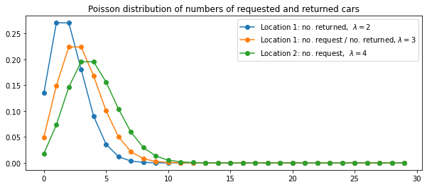
$n$ is $\frac{\lambda^n}{n!}e^{\lambda}$, where $\lambda$ is the expected number. Suppose $\lambda$ is 3 and 4 for rental requests at the first and second locations and 3 and 2 for returns. To simplify the problem slightly, we assume that there can be no more than 20 cars at each location (any additional cars are returned to the nationwide company, and thus disappear from the problem) and a maximum of five cars can be moved from one location to the other in one night. We take the discount rate to be \gamma = 0.9 and formulate this as a continuing finite MDP, where the time steps are days, the state is the number of cars at each location at the end of the day, and the actions are the net numbers of cars moved between the two locations overnight.
A Markov Decision Process (MDP) is a mathematical framework used in reinforcement learning to describe an environment. It provides a formalism to make sequential decisions under uncertainty, with an assumption that the future depends only on the current state and not on the past states. An MDP is described by a tuple (S, A, P, R), where S represents states, A represents actions, P is the state transition probability, and R is the reward function.
Using the MDP model, we can characterize Jack’s Car Rental problem as follows. The state is represented by the number of cars at each location at the end of the day, the actions correspond to the number of cars moved from location 1 to location 2, where a negative number means the cars were moved from location 2 to location 1 instead. The state transition probability depends on the number of cars rented and returned, which follow Poisson distributions. The reward function is defined by the profit made from renting cars and the cost of moving cars between locations.
A finite MDP is one in which the sets of states, actions, and rewards (S, A, and R) all have a finite number of elements. Since the states, rewards and actions are integer valued and take on a finite number of values e.g. the action is an integer between -5 and +5 , this is a finite MDP.
Let us now define the problem more formally.
The probability of ending up in state $s’$ and receiving reward $r$ given that we started in state $s$ and took action $a$, $p(s’, r \vert s, a)$, is often described in the RL book as the four argument function. It is used in the policy evaluation step of policy iteration to calculate the value of a state under a given policy.
Let us now define $p(s’, r \vert s, a)$ for this problem
Since each combination $(n_{r, 1}, n_{r, 2}, n_{b, 1}, n_{b, 2})$ is independent we can sum over their probabilities.
Let us now implement the four argument function $p(s’, r \vert s, a)$ for this problem. We will implement it in two ways. First we will implement it in a way that is easy to understand and then we will implement it in a way that is faster to run.
To start with let us import the necessary libraries and define some helper functions.
import numpy as np
import random
import pandas as pd
from scipy.stats import poisson
import itertools
import matplotlib.pyplot as plt
def get_allowed_acts(state):
# Returns the allowed actions for a given state
n1, n2 = state
acts = [0] # can always move no cars
# We can move upto 5 cars from 1 to 2
# but no more than 20-n2
# so that the total at 2 does not exceed 20
for i in range(1, min(21-n2, n1 + 1, 6)):
acts.append(i)
# The actions are defined as the number of cars moved from 1 to 2
# so if cars are moved in the opposite direction the action is negative
for i in range(1, min(21-n1, n2 + 1, 6)):
acts.append(-i)
return acts
def get_state_after_act(state, act):
# Returns the intermediate state after action
# i.e. the number of cars at each location
# after cars are moved between locations
return (min(state[0] - act, 20), min(state[1] + act, 20))
To start with let us implement the four argument function in a way that is easy to follow. We will use this to clarify our understanding of the problem and to verify the more efficient vectorised implementation that we will implement later.
def get_four_arg_iter(state, act):
First steps
Find the intermediate state after action and set up the parameters and function for the Poisson distributions.
num_after_move = get_state_after_act(state, act)
lam_b1, lam_b2 = 3, 2
lam_r1, lam_r2 = 3, 4
x1, x2 = num_after_move
def prob_fn(x, cond, lam):
# If condition is true use P(X=x), if false use 1-P(X<=x-1) = P(X >= x)
return poisson.pmf(x, mu=lam) if cond else 1 - poisson.cdf(x-1, mu=lam)
Probabilities for numbers of cars rented and added back
For each location we go through all the valid values of $n_r$ and $n_b$, calculate the next state, rental credit and the probability of $(s’, r)$ pair to which these values give rise.
location_dicts = [dict(), dict()]
for idx, (xi, lam_ri, lam_bi) in enumerate(zip((x1, x2), (lam_r1, lam_r2), (lam_b1, lam_b2))):
for nr_i in range(0, xi+1):
p_nri = prob_fn(nr_i, nr_i < xi, lam_ri)
n_space_i = 20 - (xi - nr_i)
for nb_i in range(0, n_space_i + 1):
p_nbi = prob_fn(nb_i, nb_i < n_space_i, lam_bi)
s_next_i = xi - nr_i + nb_i
location_dicts[idx][(nr_i, nb_i)] = (s_next_i, 10 * nr_i, p_nri * p_nbi)
Four argument function
Next we combine the states from the two locations, calculate the total reward and $p(s’, r|s, a, n_{b,1}, n_{b,2}, n_{r,1}, n_{r,2})$ by multiplying the probabilities from each location.
We then accumulate the probabilities for the $(s’, r)$ pairs given each combination of $n_{b,1}, n_{b,2}, n_{r,1}, n_{r,2}$ to arrive at the values of $p(s’, r|s, a)$
psrsa = dict()
move_cost = 2 * act
for (nb1, nr1), (s_next1, r1, prob1) in location_dicts[0].items():
for (nb2, nr2), (s_next2, r2, prob2) in location_dicts[1].items():
s_next = (s_next1, s_next2)
r = -move_cost + r1 + r2
key = (s_next, r)
prob = prob1 * prob2
if key not in psrsa:
psrsa[key] = prob
else:
psrsa[key] += prob
return psrsa
Whilst straightforward to understand, this implementation is quite slow as we are looping through all the valid values of $n_{r,i}$ and $n_{b,i}$ for each location.
s_init = (12, 10)
n_move = 4
%timeit get_four_arg_iter(s_init, n_move)
56.6 ms ± 3.88 ms per loop (mean ± std. dev. of 7 runs, 10 loops each)
During the policy iteration algorithm the function will be called multiple times so ideally we need a faster running time which we can achieve by vectorising the implementation.
The function will use numpy to calculate the probabilities for all pairs of requests and returns at a given location in parallel. It will then use pandas to group by the $(s’,r)$ pairs to which each $(n_{r,1}, n_{r,2}, n_{b,1}, n_{b,2})$ combination gives rise, in an efficient manner.
Let use first define a helper function that creates a unique index for each state which makes it easy to iterate though the states whilst running the algorithm.
def get_idx(s1, s2):
# Flatten the 2d state space into a 1d space
return s1 * 21 + s2
Now we can implement the four argument function in a vectorised manner.
def get_four_arg_vect(state, act):
First steps
Find the intermediate state after action and set up the parameters and function for the Poisson distributions.
num_after_move = get_state_after_act(state, act)
lam_b1, lam_b2 = 3, 2
lam_r1, lam_r2 = 3, 4
x1, x2 = num_after_move
def prob_fn(x, cond, lam):
# If condition is true use P(X=x), if false use 1-P(X<=x-1) = P(X >= x)
return np.where(cond,
poisson.pmf(x, mu=lam),
1 - poisson.cdf(x-1, mu=lam))
Probabilities and next states for each location
This is similar to the iterative implementation above but we calculate the probabilities and next states each combination of nr and nb for a given location at the same time rather than looping through them.
One subtlety is that the maximum value of $n_{b,i}$ is $20 - (x_i - n_{r,i})$ but a simple vectorised approach not involving structures like ragged arrays requires all rows of the array to have the same number of columns. To handle this we masking to filter out the invalid combinations.
location_arrs = []
for xi, lam_ri, lam_bi in zip((x1, x2), (lam_r1, lam_r2), (lam_b1, lam_b2)):
# Define nr, calculate probability of nr given xi and calculate the number of spaces for nb
# Shape: [xi + 1]
nr_i = np.arange(0, xi+1)
p_nri = prob_fn(nr_i, nr_i < xi, lam_ri)
n_space_i = 20 - (xi - nr_i)
# All the possible values of nb that can arise from a given xi
# Not all lead to valid combinations of (nr, nb) so we will mask them out later
# Note that np.max(n_space_i) = 20 - xi
# Shape: [20 - xi + 1]
nb_i = np.arange(np.max(n_space_i) + 1)
# Note that the condition is nb_i < n_space_i[:, None]
# which has shape [xi + 1, 20 - xi + 1].
# This ensures we calculate probabilities with a different upper limit for each row.
p_nbi = prob_fn(nb_i, np.less(nb_i, n_space_i[:, None]), lam_bi)
# Mask to exclude invalid combinations of (nr, nb)
# which occur when nb exceeds the number of spaces available
# Shape: [xi + 1, 20 - xi + 1]
mask_i = np.less_equal(nb_i, n_space_i[:, None])
# Select the valid pairs
nr_i, nb_i = np.where(mask_i)
# Find value of next state and probability of next state
s_next_i = xi - nr_i + nb_i
prob_nbi_nri = (p_nbi * p_nri[:, None])[mask_i]
location_arrs.append((s_next_i, nr_i, prob_nbi_nri))
Combine the states
At this point we have all the valid combinations of $(n_{r,1}, n_{b,1})$ and $(n_{r,2}, n_{b,2})$ We now combine them to get all the valid combinations of $(n_{r,1}, n_{b,1}, n_{r,2}, n_{b,2})$ and the states, rewards and probabilities that arise from them.
(s_next1, s_next2), (n_rent1, n_rent2), (prob1, prob2) = [
map(np.ravel, np.meshgrid(arr1, arr2))
for (arr1, arr2) in zip(*location_arrs)
]
n_rent = n_rent1 + n_rent2
prob = prob1 * prob2
Final Dataframe
We store the $(s’, r_c)$ rather than $(s’, r)$ pairs in the dataframe
but we can easily convert the former to the latter by subtracting the cost of moving the cars.
We saw that $p(s’, r \vert s, a)$ depends only on the intermediate state
$x = (x_1, x_2)$ so storing the values in this way let us reuse them for all the $(s, a)$ pairs that lead to given $x$.
Since the cost 2*abs(n_a) is constant for all the (s’, r) given (s, a)
the grouping in groupby will be independent of this constant offset.
Note also the probabilities in the prob
column are correct despite this offset because
as noted earlier $p(s’, r \vert s, a) = p(s’, r + 2\vert n_a \vert \vert s, a)$
df = pd.DataFrame(
{'s1': s_next1,
's2': s_next2,
'nr': n_rent,
'prob': prob
}
)
df = df.groupby(['s1', 's2', 'nr'], as_index=False).prob.sum()
df['r'] = df['nr'] * 10
# Add flat index to help iterate through states
df['idx'] = get_idx(df['s1'], df['s2'])
return df
Let us verify this method matches for the same values of s_init
and n_move
pdict_iter = get_four_arg_iter(s_init, n_move)
z = get_four_arg_vect(s_init, n_move)
pdict_vect = z.assign(rr = -2*abs(n_move) + z['r']).set_index(['s1','s2', 'rr']).to_dict()['prob']
pdict_vect = {((_s1, _s2), _r): p for (_s1, _s2, _r), p in pdict_vect.items()}
assert set(pdict_iter) == set(pdict_vect)
for i in pdict_iter:
assert np.isclose(pdict_iter[i], pdict_vect[i])
del z, pdict_vect, pdict_iter
We can also see that the function runs considerably faster than the iterative implementation.
%timeit get_four_arg_vect(s_init, n_move)
9.01 ms ± 365 µs per loop (mean ± std. dev. of 7 runs, 100 loops each)
To find an optimal policy we start with some arbitrary policy and repeat the following until convergence
Because the Jack’s car rental MDP is finite, it has only a finite number of policies which means that policy iteration must converge to an optimal policy and the optimal value function in a finite number of iterations.
To get started let us define the state space and some other values that we will need later. Since the state space is finite it can be stored in a finite array. We will use a 1d array to store the states and a dictionary to map the index of each state to the state itself. We will also define some parameters including the discount factor $\gamma$ and the threshold $\theta$ for the policy evaluation step.
state_tuples = list(itertools.product(range(21), range(21)))
state_idx = [get_idx(*s) for s in state_tuples]
states = dict(zip(state_idx, state_tuples))
gamma = 0.9
theta = 1e-6
Next we will write a helper function that finds
\[\sum_{s',r} p(s',r \vert s, a)\left[r + \gamma V(s')\right]\]The function assumes the existence of a cache where $p(s’,r \vert s, a)$ dataframes are stored keyed by the intermediate states $x$ following the action. As noted earlier we store the $(s’, r + 2\vert n_a \vert)$ rather than the $(s’, r)$ pairs in the dataframe in order to be able to use the dataframe for different $(s, a)$ pairs that give rise to the same intermediate state $x$.
For instance all the following pairs of $(s, a)$ give rise to the same $x = (19, 17)$
\[((16, 20), -3) \longrightarrow (19, 17) \\ ((17, 19), -2) \longrightarrow (19, 17) \\ ((18, 18), -1) \longrightarrow (19, 17) \\ ((19, 17), 0) \longrightarrow (19, 17) \\ ((20, 16), 1) \longrightarrow (19, 17)\]Using a cache can help avoid unnecessary calculations and speed up the running time of the algorithm.
def get_value(state, action, values, cache, gamma=0.9):
#
start = get_state_after_act(state, action)
if start not in cache:
cache[start] = get_four_arg_vect(state, action)
psrsa_df = cache[start]
# Select values of next states
V_s_next = values[psrsa_df['idx'].values].values
# Find final reward by subtracting move cost
rental_credit = psrsa_df['r'].values
move_cost = abs(action) * 2
r = rental_credit - move_cost
# Calculate value
psrsa = psrsa_df['prob'].values
val = ((gamma * V_s_next + r) * psrsa)
return val.sum()
Now will implement and run policy iteration. The algorithm statement given below is from Policy Iteration (using iterative policy evaluation) for estimating $\pi \approx \pi_*$ found in Chapter 4.3 Policy Iteration of the RL book.
1. Initialization
$V(s) \in \mathcal{R}$ and $\pi(s) \in A(s)$ arbitrarily for all $s \in \mathcal{S}$
# Also initialise a cache and a `history` array to store the intermediate results for plotting
cache = dict()
V = pd.Series(index=state_idx, data=np.zeros(len(states)))
pi = pd.Series(index=state_idx, data=np.zeros(len(states)))
delta_vals = {}
history = []
iters = 0
while True:
2. Policy Evaluation
\[\begin{aligned} &\text{Loop:} \\ &\quad \quad \Delta \leftarrow 0 \\ &\quad \quad \text{Loop for each $s \in \mathcal{S}$:} \\ &\quad \quad \quad \quad v \leftarrow V(s) \\ &\quad \quad \quad \quad V(s) \leftarrow \sum_{s', r} p\left(s',r\vert s, \pi(s)\right)\left[\gamma V(s) + r \right] \\ &\quad \quad \Delta \leftarrow \max\left(\Delta, \left\lvert v - V(s)\right\rvert\right) \\ &\text{until $\Delta < \theta$ (a small positive number determining the accuracy of estimation)} \end{aligned}\]
print('Starting Policy Evaluation')
iters += 1
policy_eval_iters = 0
delta_vals[iters] = []
while True:
delta = 0
for idx in (state_idx):
v = V[idx]
V[idx] = get_value(states[idx], pi[idx], V, cache, gamma)
delta = max(delta, abs(v - V[idx]))
policy_eval_iters += 1
sys.stdout.write('\rIteration {}, Policy Eval Iteration {}, Δ = {:.5e}'.format(iters, str(policy_eval_iters).rjust(2, ' '), delta));
delta_vals[iters].append(delta)
if delta < theta:
break
print()
print('Policy Evaluation done')
print()
3. Policy Improvement
\[\begin{aligned} &policy\text{-}stable \leftarrow true \\ &\text{For each $s \in \mathcal{S}$:} \\ &\quad \quad old\text{-}action \leftarrow \pi(s) \\ &\quad \quad \pi(s) \leftarrow \arg\max_a\sum_{s', r} p\left(s',r\vert s, a\right)\left[\gamma V(s) + r \right] \\ &\quad \quad \text{If $old\text{-}action \neq \pi(s)$, then $policy\text{-}stable \leftarrow false$} \\ &\text{If $policy\text{-}stable$ the stop and return $V \approx v_*$ and $\pi \approx \pi_*$; else go to $2$} \ \end{aligned}\]
print('Starting Policy Iteration')
policy_stable = True
history.append(pi.copy(deep=True))
for idx in (state_idx):
s = states[idx]
act = pi[idx]
actions = get_allowed_acts(s)
values_for_acts = [get_value(s, a, V, cache, gamma) for a in actions]
best_act_ind = np.argmax(values_for_acts)
pi[idx] = actions[best_act_ind]
if (act != pi[idx]):
policy_stable = False
if policy_stable:
print('Done')
break
else:
print('Policy changed - repeating eval')
print()
print('-' * 100)
Starting Policy Evaluation
Iteration 1, Policy Eval Iteration 96, Δ = 8.99483e-07
Policy Evaluation done
Starting Policy Iteration
Policy changed - repeating eval
----------------------------------------------------------------------------------------------------
Starting Policy Evaluation
Iteration 2, Policy Eval Iteration 76, Δ = 9.01651e-07
Policy Evaluation done
Starting Policy Iteration
Policy changed - repeating eval
----------------------------------------------------------------------------------------------------
Starting Policy Evaluation
Iteration 3, Policy Eval Iteration 70, Δ = 9.62239e-07
Policy Evaluation done
Starting Policy Iteration
Policy changed - repeating eval
----------------------------------------------------------------------------------------------------
Starting Policy Evaluation
Iteration 4, Policy Eval Iteration 52, Δ = 8.39798e-07
Policy Evaluation done
Starting Policy Iteration
Policy changed - repeating eval
----------------------------------------------------------------------------------------------------
Starting Policy Evaluation
Iteration 5, Policy Eval Iteration 17, Δ = 7.18887e-07
Policy Evaluation done
Starting Policy Iteration
Done
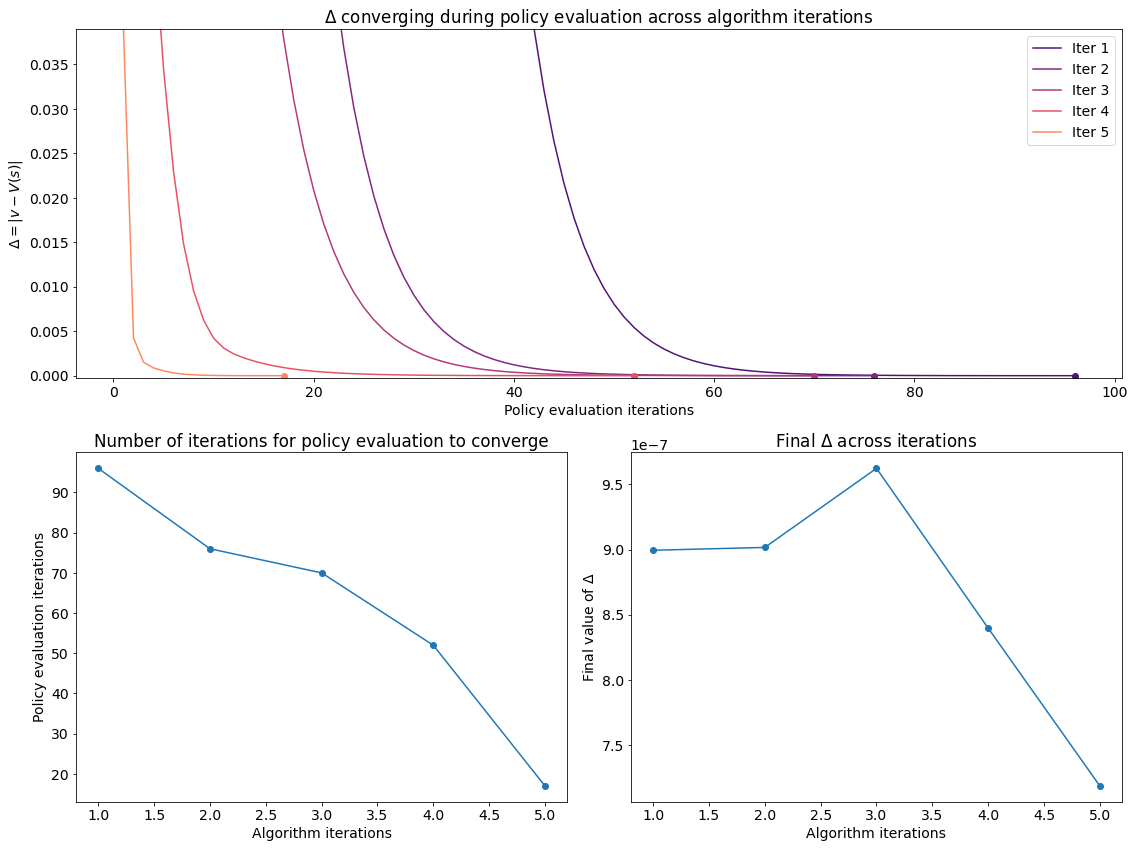
We can visualise the progress of the algorithm in the plots below. Evidently policy evaluation converges faster across iterations of the algorithm and after the first few iterations attains a lower final value.
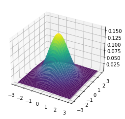
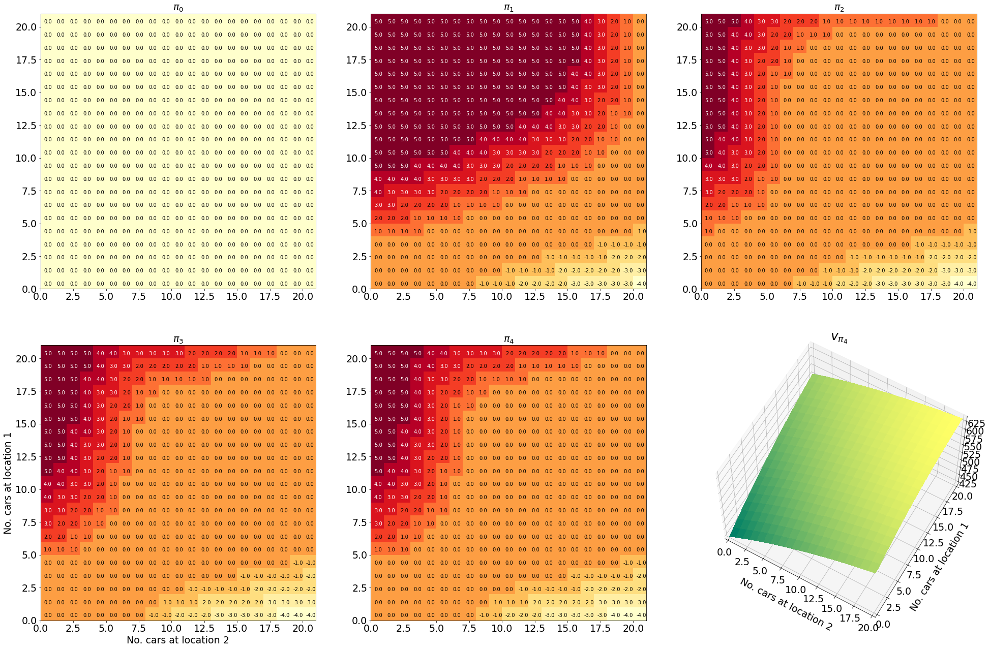
Having successfully run the algorithm, let us visualise the results by creating a figure similar to Figure 4.2 in the RL book. The figure shows the initial policy $\pi_0$ and the policy after each iteration as a heatmap for each combination of the number of cars at each location, $(s_1, s_2)$. It also shows the value function $v_{\pi_4}$ as a 3D plot for each state.
The policies are in a flattened form so we reshape them into a 2D grid for plotting the results in the form of heatmaps. We also reshape the states and values into 21x21
pi_grid = np.reshape([pi[i] for i in state_idx], (21, 21))
idx_grid = np.reshape([states[i] for i in state_idx], (21, 21, 2))
V_grid = np.reshape([V[i] for i in state_idx], (21, 21))
Here is a helper function that adds text labels to the grid. The function takes the states, values, mask and offsets for the text labels as arguments. It also takes a threshold and a boolean lower
which determines whether the mask is applied to values lower or higher than the threshold. The function then plots the values as text on the grid, with the text colour set to white if the mask is satisfied and black otherwise.
def plot_grid(states, values, mask, offx, offy, th, axis=None, lower=True):
# Assumes a colormesh has already been plotted on the axis
# and adds text labels to the grid
axis = plt.gca() if axis is None else axis
for state, value, m in zip(states, values, mask):
axis.text(state[1]+offx,state[0]+offy,value,
color='white' if (m < th if lower else m > th) else 'k')
Finally let us make the plots. The plots are arranged in a 2x3 grid. The first 5 plots show the policies $\pi_0, \pi_1, \pi_2, \pi_3, \pi_4$ and the last plot shows the value function $v_{\pi_4}$.
fig = plt.figure(figsize=(33, 22))
gs = plt.GridSpec(2, 3)
fontsize = 19
cmap = 'YlOrRd'
for t in range(len(history) + 1):
if t < 5:
pi_grid_i = np.reshape([history[t][i] for i in state_idx], (21, 21))
axis = plt.subplot(gs[t])
axis.pcolormesh(pi_grid_i, cmap=cmap)
plot_grid(
idx_grid.reshape([-1, 2]),
pi_grid_i.reshape([-1]),
.25, .25, 2, axis=axis, lower=False
)
axis.set_aspect('equal', adjustable='box')
axis.set_title(f'$\pi_{t}$', fontsize=fontsize)
else:
axis = plt.subplot(gs[-1], projection='3d')
X = idx_grid[..., 1]
Y = idx_grid[..., 0]
Z = V_grid
axis.plot_surface(X, Y, Z, cmap='summer', linewidth=0, antialiased=False)
axis.view_init(60, -60)
axis.set_xlim([0, 20])
axis.set_ylim([0, 20]);
axis.set_title('$v_{\\pi_4}$', fontsize=25)
if t in [3, 5]:
space = '\n'*2 if t == 5 else ''
axis.set_ylabel(f'{space}No. cars at location 1', fontsize=fontsize)
axis.set_xlabel(f'{space}No. cars at location 2', fontsize=fontsize)
axis.tick_params(labelsize=fontsize)
Here is an animated version showing how the algorithm progresses towards the final result
And here is an interactive version of the final state-value function
In this tutorial, we will discuss various ways to use curly brackets $\{\}$ in LaTeX. The simplest case involves using curly brackets to denote a set e.g. $\{x, y, z\}$ is the set containing the elements $x$, $y$ and $z$. However, curly brackets, or braces, can also be used to group multiple lines of calculations and mathematical equations or to add explanatory text above or below the expressions.
As an added bonus, some of the examples in this tutorial come from the Denoising Diffusion Probabilistic Model (DDPM) paper. You can find a tutorial about the DDPM paper here.
Curly brackets have a special meaning in LaTeX. They are used grouping and delimiting the scope of commands, allowing you to apply formatting or modifications to specific portions of text or to define the extent of arguments for commands.
For example “\sqrt{2x}” would render as the square root of the expression $2x$, $\sqrt{2x}$ while “\sqrt 2x” would render as the square root of “2” times “x”, $\sqrt 2x$. Here, the curly brackets are used to define the extent of the argument for the square root command.
To display the curly brackets themselves, we need to use the escape characters \{
and \}
. If we simply write {x, y, z}
, it will be interpreted as a grouping of x, y, z
and rendered as $x, y, z$.
To display the curly brackets, we should write \{x, y, z\}
. This will be rendered as $\{x, y, z\}$.
In some cases, we may need to adjust the size of the curly brackets to match the size of the content inside them. This can be done using the \left
and \right
commands. These commands automatically resize the brackets based on the height of the content.
Without using \left
and \right
{\frac{1}{4}, \frac{1}{2}, 1\}
renders as
\[\{\frac{1}{4}, \frac{1}{2}, 1\}\]where the fractions are not properly enclosed by the brackets.
Using \left and \right we can write
\left\{\frac{1}{4}, \frac{1}{2}, 1\right\}
which renders as
\[\left\{\frac{1}{4}, \frac{1}{2}, 1\right\}\]which is more aesthetically pleasing and easier-to-read expression.
In LaTeX, you can easily group multiple lines together with the align
environment. Insert the \begin{align}
and \end{align}
commands to start and end the aligning of your lines respectively. Then, use curly braces to enclose the portions you wish to group together and the &
symbol to align around equals or other operators.
The general syntax is as follows:
\left\{
\begin{aligned}
& expression1 \\
& expression2 \\
& expression3 \\
& expression4 \\
\end{aligned}
\right.
Breakdown of the syntax:
\left\{ and \right.
: These commands create the curly braces that enclose the expressions.\begin{aligned}
and \end{aligned}
: These commands create the align environment.&
: This symbol aligns the expressions vertically.Below is an example that breaks down the calculation of an absolute value into several parts:
\begin{align*}
|x| =
\left\{
\begin {aligned}
& x \quad & x \geq 0 \\
& -x \quad & x < 0
\end{aligned}
\right.
\end{align*}
which produces the following output:
\[\begin{align*} |x| = \left\{ \begin {aligned} & x \quad & x \geq 0 \\ & -x \quad & x < 0 \end{aligned} \right. \end{align*}\]Here we have also introduced additional syntax to format each line of the equation.
& case1 \quad &\condition1
where the \quad
command adds a space between the two expressions. The &
symbol after \quad
aligns the conditions vertically.
The final transition distribution of the reverse process $p_\theta\left(\mathbf{x}_0 \vert \mathbf{x}_1\right)$, which denotes the transition from the final latent $\mathbf{x}_1$ is modelled as an independent decoder. The data $\mathbf{x}_0$ is assumed to consists of integers $0,1,\ldots,255$, linearly scaled to lie in the interval $[−1,1]$. The form of the distribution for the last term of the reverse process is given by the products of the element-wise distributions
\[p_\theta\left(\mathbf{x}_0 \vert \mathbf{x}_1\right) = \prod_{i=1}^D\int_{\delta_{-}\left(x_0^i\right)}^{\delta_{+}\left(x_0^i\right)} \mathcal{N}\left(x; \mu_\theta^i\left(\mathbf{x}_1, 1\right), \sigma_1^2\right)dx \\ \delta_{+}(x)= \left\{ \begin{aligned} &\infty \quad & x = 1 \\ &x + \frac{1}{255} \quad& x < 1 \\ \end{aligned} \right. \\ \delta_{-}(x)= \left\{ \begin{aligned} &-\infty \quad & x = 1 \\ &x - \frac{1}{255} \quad& x < 1 \\ \end{aligned} \right.\]where the delta terms are written using multi-line braces e.g. for $\delta_{+}(x)$ the latex code is:
\begin{aligned}
&\infty \quad & x = 1 \\
&x + \frac{1}{255} \quad& x < 1 \\
\end{aligned}
You can also group a subset of lines together with the align
environment. Insert the \begin{align}
and \end{align}
commands to start and end the aligning of your lines respectively. Then, use curly braces to enclose the portions you wish to group together and the &
symbol to align around equals or other operators.
The general syntax is as follows:
\begin{align*}
expression1 \\
expression2 \\
\left.
\begin{aligned}
& expression3 \\
& expression4 \\
\end{aligned}
\right\} \quad & \text{Group 1} \\
expression5 \\
expression6 \\
Below is an example that breaks down the calculation of the Fibonacci sequence into the base cases and the recursive case. The two base cases are grouped together with the align
environment and the recursive case is placed outside of the environment.
\begin{align*}
\left.
\begin{aligned}
& F(0) = 0 \\
& F(1) = 1 \\
\end{aligned}
\right\} \quad & \text{Base cases} \\
F(n) = F(n-1) + F(n-2) \quad & \text{Recursive case}
\end{align*}
which produces the following output:
\[\begin{align*} \left. \begin{aligned} & F(0) = 0 \\ & F(1) = 1 \\ \end{aligned} \right\} \quad & \text{Base cases} \\ F(n) = F(n-1) + F(n-2) \quad & \text{Recursive case} \end{align*}\]Another handy function includes the overbrace and underbrace which enables you to add explanatory text above or below the expressions you wish to highlight.
The general syntax is as follows:
Overbrace: \overbrace{expression}^{explanation}
Underbrace: \underbrace{expression}_{explanation}
Here is an example of an equation with three terms, each explained by an underbrace:
f(x)= \underbrace{3x^2}_{\text{quadratic term}} + \underbrace{2x}_{\text{linear term}} + \underbrace{1}_{\text{constant}}
which produces the following output:
\[f(x)= \underbrace{3x^2}_{\text{quadratic term}} + \underbrace{2x}_{\text{linear term}} + \underbrace{1}_{\text{constant}}\]The following example groups the linear and quadratic terms together using an overbrace:
f(x) = \overbrace{3x^2 + 2x}^{\text{terms which depend on } x} + 1
which produces the following output:
\[f(x) = \overbrace{3x^2 + 2x}^{\text{terms which depend on } x} + 1\]overbrace
and underbrace
We may also use a combination of overbrace
and underbrace
for example here an overbrace encloses an expression with two underbraces
f(x) = \overbrace{\underbrace{3x^2}_{\text{quadratic term}} + \underbrace{2x}_{\text{linear term}}}^{\text{terms which depend on } x} + \underbrace{1}_{\text{constant}}
which would render as
\[f(x) = \overbrace{\underbrace{3x^2}_{\text{quadratic term}} + \underbrace{2x}_{\text{linear term}}}^{\text{terms which depend on } x} + \underbrace{1}_{\text{constant}}\]It can be shown that the loss function can be written as follows
\[\mathbb{E}_q\left[\underbrace{\text{D}_\text{KL}\left(q(\mathbf{x}_T|\mathbf{x}_0\right) \Vert p(\mathbf{x}_T))}_{L_T} + \overbrace{\sum_{t>1} \underbrace{\text{D}_\text{KL}\left(q(\mathbf{x}_{t-1}|\mathbf{x}_t, \mathbf{x}_0\right) \Vert p_\theta(\mathbf{x}_{t-1}|\mathbf{x}_0))}_{L_{t-1}} \underbrace{- \log p_{\theta} (\mathbf{x}_0 | \mathbf{x}_1}_{L_0})}^{\text{terms which depend on }\theta}\right]\]To summarise, we have explored how to use braces in LaTeX. We have discussed the align
environment for grouping multiple lines together and the syntax for creating multi-line braces using curly brackets. Additionally, we have learned about the \overbrace
and \underbrace
functions that allow us to add explanatory text above or below expressions. These techniques will be useful when writing complex mathematical equations and calculations in LaTeX.
A windrose, or a polar rose plot, is polar histogram that shows the distribution of wind speeds and directions over a period of time. It is a useful tool for visualising how wind speed and direction are typically distributed at a given location. The data is divided into direction intervals, and the frequency of wind speeds in each direction is represented by the radius of the bars. Typically the data is also binned into speed intervals and plotted as a set of stacked bars, where each bar represents a speed interval. The height of the bar is the frequency of wind speeds in that interval, and the radius of the bar is the sum of the frequencies of wind speeds in that interval.
In this tutorial we will learn:
This blogpost can be found as a Colab notebook here.
The data used in this tutorial is available here. To following along download it and replace filepath
below with the location at which you saved the data.
We have a dataframe containing wind speed and direction data measured at Coimbatore airport in India.
SPD
- wind speed in m/sDIR
- wind direction in degreesMM
- month of the year between 1 and 12Let us take a look at the first few rows of the data:
import calendar
import pandas as pd
import numpy as np
import matplotlib.pyplot as plt
# Modify to point to location where your data is saved
filepath = 'coimbatore-airport-2016.csv'
# Load data
df = pd.read_csv(filepath)
# Display the first few rows of the dataframe
df.head()
NAME | HR_TIME | YYYY | MM | DD | HR | MN | TEMP | DEWP | SPD | DIR | |
---|---|---|---|---|---|---|---|---|---|---|---|
0 | 433210-99999 | 2016010100 | 2016 | 1 | 1 | 0 | 0 | 65 | 62 | 5 | 360 |
1 | 433210-99999 | 2016010100 | 2016 | 1 | 1 | 0 | 0 | 64 | 63 | 5 | 360 |
2 | 433210-99999 | 2016010100 | 2016 | 1 | 1 | 0 | 30 | 64 | 63 | 3 | 360 |
3 | 433210-99999 | 2016010101 | 2016 | 1 | 1 | 1 | 0 | 64 | 63 | 3 | 360 |
4 | 433210-99999 | 2016010102 | 2016 | 1 | 1 | 2 | 30 | 66 | 63 | 3 | 20 |
First, we need to transform our raw wind data, which is a crucial step in constructing a windrose plot.
The windrose_histogram
function partitions the raw wind speed and direction data into bins, counts the frequency of observations in each bin, and optionally normalizes these frequencies. The result is a 2D histogram, ideal for creating windrose plots.
def windrose_histogram(wspd, wdir, speed_bins=12, normed=False, norm_axis=None):
"""
Compute a windrose histogram given wind speed and direction data.
wspd: array of wind speeds
wdir: array of wind directions
speed_bins: Integer or Sequence, defines the bin edges for the wind speed (default is 12 equally spaced bins)
normed: Boolean, optional, whether to normalize the histogram values. (default is False)
norm_axis: Integer, optional, the axis along which the histograms are normalized (default is None)
"""
# If speed_bins is an integer, we create linearly spaced bins from 0 to max speed
if isinstance(speed_bins, int):
speed_bins = np.linspace(0, wspd.max(), speed_bins)
num_spd = len(speed_bins)
num_angle = 16
# Shift wind directions by 11.25 degrees (one sector) to ensure proper alignment
wdir_shifted = (wdir + 11.25) % 360
angle_bins = np.linspace(0, 360, num_angle + 1)
# Generate a 2D histogram using the defined speeds bins and shifted wind directions
hist, *_ = np.histogram2d(wspd, wdir_shifted, bins=(speed_bins, angle_bins))
# Normalize if required
if normed:
hist /= hist.sum(axis=norm_axis, keepdims=True)
hist *= 100
return hist, angle_bins, speed_bins
This windrose_histogram
function partitions the wind speed and direction data into bins, counts the frequency of observations in each bin, and optionally normalizes these frequencies. The result is a 2D histogram, ideal for creating windrose plots.
Before diving into the intricacies of windrose plotting, we must first transform our raw wind data into a structured format that is more suitable for analysis. To achieve this, we’ll employ the following function:
DIRECTION_NAMES = ("N","NNE","NE","ENE"
,"E","ESE","SE","SSE"
,"S","SSW","SW","WSW"
,"W","WNW","NW","NNW")
DIRECTION_ANGLES = np.arange(0, 2*np.pi, 2*np.pi/16)
# Mapping from direction name to angles in radians
NAME2ANGLE = dict(zip(
DIRECTION_NAMES,
DIRECTION_ANGLES
))
def make_wind_df(data_df, num_partitions, max_speed=None, normed=False, norm_axis=None, month=None):
"""
This function transforms raw wind speed and direction data into a DataFrame for windrose plotting.
data_df: Dataframe containing wind data
num_partitions: Integer, number of partitions to divide the wind speed data
max_speed: Float, optional, maximum wind speed to be included in the partitions
normed: Boolean, optional, whether to normalize the frequency values
norm_axis: Integer, optional, the axis along which the histograms are normalized
"""
if month is not None:
data_df = data_df[data_df.MM==month]
wspd = data_df['SPD'].values
wdir = data_df['DIR'].values
# If max_speed is not specified, we use the maximum value in the 'wspd' data.
# Otherwise, we include all speeds up to and including max_speed.
# Additional partitions are created to handle outliers.
if max_speed is None:
speed_bins = np.linspace(0, wspd.max(), num_partitions + 1)
else:
speed_bins = np.append(np.linspace(0, max_speed, num_partitions + 1), np.inf)
# windrose_histogram function is called to partition data based on the bins created.
# Additional parameters control how the frequency values are normalised
h, *_ = windrose_histogram(wspd, wdir, speed_bins, normed=normed, norm_axis=norm_axis)
# A dataframe is formed containing the histogram data. Column names are for the directions
wind_df = pd.DataFrame(data=h, columns=DIRECTION_NAMES)
# speed_bin_names stores speed range strings to describe each interval
# e.g. when speed_bins is [0, 3, 6], speed_bin_names is ['0-3', '3-6', '>6']
speed_bin_names = []
speed_bins_rounded = [round(i, 2) for i in speed_bins]
for start, end in zip(speed_bins_rounded[:-1], speed_bins_rounded[1:]):
speed_bin_names.append(f'{start:g}-{end:g}' if end < np.inf else f'>{start:g}')
wind_df['strength'] = speed_bin_names
# Reshapes data for plotting. Now, each row represents one sector of the windrose
wind_df = wind_df.melt(id_vars=['strength'], var_name='direction', value_name='frequency')
return wind_df
Here is what the dataframe looks like
make_wind_df(df, num_partitions=4).head(12)
strength | direction | frequency | |
---|---|---|---|
0 | 0-6.25 | N | 189.0 |
1 | 6.25-12.5 | N | 14.0 |
2 | 12.5-18.75 | N | 0.0 |
3 | 18.75-25 | N | 0.0 |
4 | 0-6.25 | NNE | 648.0 |
5 | 6.25-12.5 | NNE | 145.0 |
6 | 12.5-18.75 | NNE | 1.0 |
7 | 18.75-25 | NNE | 0.0 |
8 | 0-6.25 | NE | 815.0 |
9 | 6.25-12.5 | NE | 389.0 |
10 | 12.5-18.75 | NE | 15.0 |
11 | 18.75-25 | NE | 0.0 |
Matplotlib is a versatile and comprehensive library in Python that allows for a wide variety of plotting types, such as scatter plots, bar charts, and line charts.
While Matplotlib does not have out-of-the-box capabilities to create a windrose, thanks to the library’s flexibility, we can make a plot which resembles a windrose using polar bar diagrams, where the height of the bars demonstrates the frequency of the wind speed, and the orientation of the bars represents the wind direction.
A polar plot is a diagram in which data points are represented in a polar coordinate system. In this system, a point’s location is determined by its distance from the centre (known as the radial coordinate $\rho$ or $r$) and by the angle from a reference direction (known as the angular coordinate $\phi$ or $\theta$).
Here is an example of a polar plot which shows an Archimedean spiral which can be represented by a linear polar equation
\[r(\phi) = a + b\phi\]We plot it with
\[a = 0, b = \frac{1}{2\pi} \quad \text{and} \quad a = 2, b = \frac{1}{4\pi}\]phi = np.linspace(0, 10*np.pi, 1001)
avals = [0, 2]
bvals = [1/(2*np.pi), 1/(4*np.pi)]
blabels = ['2\pi', '4\pi']
fig, axes = plt.subplots(1, 2, subplot_kw={'projection': 'polar'}, figsize=(10,4))
for clr, axis, a, b, bl in zip(['mediumblue', 'darkorange'], axes, avals, bvals, blabels):
axis.plot(phi, a + b*phi, linewidth=2, color=clr);
axis.set_title(f'$r(\phi) = {(str(a) + " + ") if a > 0 else ""}'
+"\\frac{\phi}{" + f'{bl}' +' }$' )
plt.suptitle(' Archimedean spirals');
In the context of windroses, we use polar plots for illustrating the wind direction (angular coordinate) and the wind speed (radial coordinate).
def matplotlib_windrose(data_df, num_partitions=4, max_speed=4, month=None):
"""
Function to create a windrose plot using matplotlib.
Args:
data_df: Dataframe containing wind data
num_partitions: number of partitions for wind strength
max_speed: maximum wind speed to be considered while partitioning the wind strength
month: (optional) a string representing the month, used in defining the DataFrame for plotting
Returns:
fig: a matplotlib Figure object containing the windrose plot
"""
# calls the make_wind_df function to create a dataframe which
# reshapes raw wind speed and direction data for windrose plotting
wind_df2 = make_wind_df(data_df=data_df,
num_partitions=num_partitions,
max_speed=max_speed,
normed=True,
month=month)
wind_df2['frequency'] = wind_df2['frequency']/ 100
# modifies the dataframe by extracting start strength based on certain conditions in each strength value
wind_df2 = wind_df2.assign(strength_start=[float(x.split('-')[0] if '-' in x else x[1:])
for x in wind_df2.strength.values])
# converts the mapped direction names to angles and sorts the dataframe according to the strength start
wind_df2['angle'] = wind_df2.direction.map(NAME2ANGLE)
wind_df2 = wind_df2.sort_values(by='strength_start')
# The command below does three things sequentially:
# 1. It sorts the dataframe 'wind_df2' in ascending order according to 'strength_start'.
# 2. It groups this sorted dataframe by 'direction' so the each group contains the sorted values of 'strength_start' for the corresponding direction.
# 3. It cumulatively sums the frequencies within each group (i.e., each unique wind direction) direction.
# The cumulative frequency value for a given strength_start value is the sum of the frequencies of all the strength_start values that are less than or equal to the given strength_start value. The reason for doing this is to enable us to plot stacked bars in the windrose plot.
wind_df2['cumulative_frequency'] = wind_df2.sort_values(by='strength_start').groupby('direction').frequency.cumsum()
# Use black background
with plt.style.context('dark_background'):
# create a polar plot (windrose) with given figure size
fig, axis = plt.subplots(figsize=(8, 8), ncols=1, subplot_kw=dict(projection="polar"))
# adds a grid to the plot in white since background will be dark
axis.grid(color='white')
# extracts values from the 'strength_start' column of the dataframe
strength_starts = wind_df2.strength_start.values
# defines the colormap to be used for different strength partitions in the windrose
colours = plt.cm.magma_r(
np.linspace(0, 1, wind_df2.strength.nunique())
)
# groups the dataframe by 'strength'
strength_splits = wind_df2.groupby('strength')
# plots a bar chart for each unique strength value in the windrose plot
# in descending order of strength to make the bars appear stacked on top of each other
# since the frequency values are cumulative, the bars are stacked on top of each other
for clr, strength in list(zip(colours, wind_df2.strength.unique()))[::-1]:
split = strength_splits.get_group(strength)
# Note that the width is slightly less than 22.5 degrees (i.e., 360/16) so that the bars are slightly separated from each other which makes the plot look better
# zorder=2 ensures grid does not appear on top of the bars
axis.bar(split['angle'].values,
split['cumulative_frequency'].values,
color=clr,
label=strength,
width=np.deg2rad(19),
edgecolor='black',
linewidth=0.5,
zorder=2)
# sets direction names as xticks in the windrose plot
axis.set_xticks(DIRECTION_ANGLES)
axis.set_xticklabels(DIRECTION_NAMES)
# adds a legend to the plot
handles, labels = axis.get_legend_handles_labels()
axis.legend(
handles[::-1],
labels[::-1],
loc='upper left',
bbox_to_anchor=(1.1, 1.1)
);
# sets the zero location of the theta axis to North
axis.set_theta_zero_location('N')
# sets the direction of the theta axis to clockwise (-1)
axis.set_theta_direction(-1)
axis.set_title('Wind rose ({})'.format(
calendar.month_name[month] if month in range(1, 13) else 'Annual'
))
axis.set_rlabel_position(135)
yticks = axis.get_yticks()
ytick_labels = [('{:.2f}'.format(round(i * 100, 2))[:-1]).rstrip('0').rstrip('.') + '%' for i in yticks]
axis.set_yticks( yticks)
axis.set_yticklabels(ytick_labels)
# returns the figure containing the windrose plot
return fig
To use the matplotlib_windrose
function, you pass in the wind dataframe plus additional arguments to vary the appearance of the plot. Below we shall see how to add interactivity so that we can vary these parameters and update the plot each time.
matplotlib_windrose(df, num_partitions=8, max_speed=25);
For an alternative approach, we turn to Plotly, another Python library known for its advanced plotting capabilities. We can leverage Plotly Express to achieve a straightforward realisation of a windrose plot.
The plotly_windrose
function operates similarly to the make_wind_df
function but utilizing Plotly’s ‘px.bar_polar’ to create the windrose plot, enhancing the plot with interactive capabilities.
import plotly.express as px
def plotly_windrose(data_df, num_partitions=4, max_speed=4, month=None):
"""
Function to generate a windrose plot using Plotly.
Args:
data_df: Dataframe containing wind data
num_partitions: number of partitions for wind strength
max_speed: maximum wind speed to be considered while partitioning the wind strength
month: (optional) a string representing the month, used in defining the DataFrame for plotting
Returns:
plot: a Plotly Figure object containing the windrose plot
"""
# Convert raw data into a windrose-friendly format
wind_df = make_wind_df(data_df=data_df,
num_partitions=num_partitions,
max_speed=max_speed,
normed=True,
month=month
)
# Normalize frequency to a percentage
wind_df['frequency'] = wind_df['frequency'] / 100
# Sort strength bins in order
strengths = sorted(wind_df.strength.unique(), key=lambda x:float(x.split('-')[0] if '-' in x else x[1:]))
# defines the colormap to be used for different strength partitions in the windrose
colours =px.colors.sample_colorscale(px.colors.get_colorscale('Magma_r'), len(strengths))
colour_dict = dict(zip(strengths, colours))
# Create a polar bar plot with the specified properties
fig = px.bar_polar(wind_df, r="frequency", theta="direction",
color="strength",
color_discrete_map=colour_dict,
template="plotly_dark",
title='Wind rose ({})'.format(
calendar.month_name[month] if month in range(1, 13) else 'Annual'
)
)
# Update the polar plot parameters to enhance readability and esthetics
fig.update_polars(
radialaxis_angle = -45, # To rotate the radial axis
radialaxis_tickangle=-45, # To rotate the tick labels on radial axis
radialaxis_tickformat=',.0%', # To change the tick labels to percentages
radialaxis_tickfont_color='white', # To change tick labels to white for better readability,
)
# Make figure square
fig.update_layout(
autosize=False, # To prevent automatic adjustment of figure size
width=500, # To set figure width to 500 pixels
height=500, # To set figure height to 500 pixels
)
return fig
Creating a plot with plotly_windrose
we can see that it looks very similar to the previous plot but with Plotly’s interactive features.
plotly_windrose(df, num_partitions=8, max_speed=25)
The plots so far have shown windroses using the entire dataset. However, wind patterns can vary significantly depending on the time of year. We can use Jupyter widgets to create an interactive windrose that allows us to select the month of the year to plot.
In addition, we can also choose the number of partitions and the maximum wind speed to be included in the plot. These settings will give use greater control over the appearance of the windrose.
Widgets are interactive controls for python within Jupyter notebooks, allowing you to dynamically change variables and view the changes in output.
To create an interactive widget, we can use the interact function of the ipywidgets
library. The interact function automatically creates user interface (UI) controls for function arguments, and then calls the function with those arguments when you manipulate the controls interactively.
In addition our widget will let us choose which of the two plotting libraries we want to use, Matplotlib or Plotly.
from ipywidgets import interact, fixed, IntSlider, Dropdown, Layout, Output
month_dict = {('Annual' if i == 0 else calendar.month_name[i]):i for
i in range(13)}
def interactive_windrose(num_partitions, max_speed, month, method):
fn = {'Plotly': plotly_windrose, 'Matplotlib': matplotlib_windrose}[method]
f = fn(df, num_partitions=num_partitions,
max_speed=max_speed, month=month if month > 0 else None)
if method == 'Plotly':
f.show()
interact(interactive_windrose,
num_partitions=IntSlider(value=5, min=2, max=33, description='No. partitions',
layout=Layout(width='400px'),
style=dict(description_width='initial')),
max_speed=IntSlider(value=17, min=2, max=33, description='Max wind speed (m/s)',
layout=Layout(width='450px'),
style=dict(description_width='initial')),
month=Dropdown(options=month_dict, value=3, description='Month',
layout=Layout(margin="0px 0px 10px 0px"),
style=dict(description_width='initial')),
method=Dropdown(options=['Plotly', 'Matplotlib'], value='Plotly', description='Method',
layout=Layout(margin="0px 0px 25px 0px"),
style=dict(description_width='initial'))
);
This is what the widget looks like. You can try it out for yourself in the Colab for this blog.
In this tutorial, we have walked through the process of plotting a windrose, a polar plot which shows the distribution of wind speeds and directions over time. We covered the essential knowledge behind windroses, walked through some methods of data preparation, and learned to generate windroses using two notable Python libraries - Matplotlib and Plotly. Furthermore, we touched upon how to add interactivity to our windrose plots with Jupyter widgets, enhancing their usefulnesses. The techniques covered in this tutorial can be leveraged in meteorology, climate studies, aviation and other fields requiring wind data analysis and visualisation.
]]>When you send a message to ChatGPT you start seeing its answer within a moment. Instead of waiting for the model to produce the full answer before displaying the output, the app prints out the tokens in sequence, giving you the feel of a real-time conversation. In this blog post we will look at how you can replicate this experience using the API by streaming the response. To follow along make sure you have signed up for an OpenAI API account and have installed the openai
library that lets you use Python to make API calls (pip install openai
).
Let’s get started by asking ChatGPT to write a function to make a 3D plot of a 2D Gaussian distribution. It is not too difficult but the answer will be several lines in length. It is highly unlikely be generated almost instantly which makes it a suitable input to use for comparing the user experience with and without streaming.
When you make an API call to ChatGPT with stream
set to False
(the default option) you get back that looks something this:
<OpenAIObject chat.completion id=chatcmpl-7eijdlu4SYVIczkFfRVZMd7tZEURH at 0x108259ef0> JSON: {
"choices": [
{
"finish_reason": "stop",
"index": 0,
"message": {
"content": "Here's a Python function ...",
"role": "assistant"
}
}
],
"created": 1689939437,
"id": "chatcmpl-7eijdlu4SYVIczkFfRVZMd7tZEURH",
"model": "gpt-4-0613",
"object": "chat.completion",
"usage": {
"completion_tokens": 370,
"prompt_tokens": 63,
"total_tokens": 433
}
}
The response contains the entirety of the text output by ChatGPT in response['choices'][0]['messages']['content']
(throughout we assume only one choice of output is generated).
import time
import openai
question = ("Write a Python function `plot_2d_normal` which makes a 3D plot of a 2D Gaussian distribution with arguments `sigma` and `mu`. "
"By default it should plot a 2D standard normal.")
print(question)
Write a Python function `plot_2d_normal` which makes a 3D plot of a 2D Gaussian distribution with arguments `sigma` and `mu`. By default it should plot a 2D standard normal.
# record start time to calculate total time to get response
start_time = time.time()
response = openai.ChatCompletion.create(
model="gpt-4",
messages=[
{"role": "system", "content": "You are a helpful assistant."},
{"role": "user", "content": question}
]
)
response_time = time.time() - start_time
print(f"Full response received {response_time:.2f} seconds after request")
print('\n\nResponse:\n')
print(response['choices'][0]['message']['content'])
Full response received 31.49 seconds after request
Response:
Here's a Python function that will generate this 3D plot:
```python
from mpl_toolkits.mplot3d import Axes3D
import matplotlib.pyplot as plt
import numpy as np
def plot_2d_normal(sigma=np.array([[1, 0], [0, 1]]), mu=np.array([0, 0])):
# Define the 2d normal distribution
def p(x, y):
det_sigma = np.linalg.det(sigma)
inv_sigma = np.linalg.inv(sigma)
weight = 1.0 / (2.0 * np.pi * np.sqrt(det_sigma))
vec = np.array([x - mu[0], y - mu[1]])
return weight * np.exp(-0.5 * np.dot(vec.T, np.dot(inv_sigma, vec)))
# Create a grid of x, y values
x = np.linspace(-3, 3, 100)
y = np.linspace(-3, 3, 100)
x, y = np.meshgrid(x, y)
# Get the z values from the 2d normal distribution
z = np.vectorize(p)(x, y)
# Create the 3d plot
fig = plt.figure()
ax = fig.add_subplot(111, projection='3d')
ax.plot_surface(x, y, z, cmap='viridis')
plt.show()
plot_2d_normal()
```
By default this function plots a 2D standard normal, but you can input any `sigma` and `mu` values to change the standard deviation and mean of the distribution, respectively. This function uses the `matplotlib` library to plot the 3D Gaussian, and `numpy` to generate the grid of x and y values.
With stream
set to the default value of False
the response can take a while to be returned making for a less pleasant user experience. Here it took nearly 30 seconds.
Traditionally you get data from an API by making a request and getting a response. That is what we have done above. But setting stream true causes the response to be sent back a few chunks at a time via an event stream. In contrast to a regular API call, with an event stream, you make a request and get a response, but then the server keeps the connection open and sends you new data as it becomes available without you having to make any additional requests.
In the case of ChatGPT, instead of receiving the entire response in one go, the event stream enables us to receive the response gradually, chunk by chunk, so that can start reading the response quite quickly.
The chunks have a field delta
which shares a similar structure to message
. It can have fields like
role
of the assistantcontent
of the messageor it can be empty ({}
) when the stream is over. However the content
field contains a part of the response rather than the full response.
Here is an example of a sequence of chunks corresponds to a message that starts with “Sure,” where the the final chunk has an empty delta
field:
[<OpenAIObject chat.completion.chunk id=chatcmpl-7el59DFH8bYJWFZE6KeEkdyYNNV3a at 0x13148be00> JSON: {
"choices": [
{
"delta": {
"content": "",
"role": "assistant"
},
"finish_reason": null,
"index": 0
}
],
"created": 1689948459,
"id": "chatcmpl-7el59DFH8bYJWFZE6KeEkdyYNNV3a",
"model": "gpt-4-0613",
"object": "chat.completion.chunk"
},
<OpenAIObject chat.completion.chunk id=chatcmpl-7el59DFH8bYJWFZE6KeEkdyYNNV3a at 0x1327cbc20> JSON: {
"choices": [
{
"delta": {
"content": "Sure"
},
"finish_reason": null,
"index": 0
}
],
"created": 1689948459,
"id": "chatcmpl-7el59DFH8bYJWFZE6KeEkdyYNNV3a",
"model": "gpt-4-0613",
"object": "chat.completion.chunk"
},
<OpenAIObject chat.completion.chunk id=chatcmpl-7el59DFH8bYJWFZE6KeEkdyYNNV3a at 0x1327cb130> JSON: {
"choices": [
{
"delta": {
"content": ","
},
"finish_reason": null,
"index": 0
}
],
"created": 1689948459,
"id": "chatcmpl-7el59DFH8bYJWFZE6KeEkdyYNNV3a",
"model": "gpt-4-0613",
"object": "chat.completion.chunk"
}],
...
<OpenAIObject chat.completion.chunk id=chatcmpl-7el59DFH8bYJWFZE6KeEkdyYNNV3a at 0x1354b9220> JSON: {
"choices": [
{
"delta": {},
"finish_reason": "stop",
"index": 0
}
],
"created": 1689948459,
"id": "chatcmpl-7el59DFH8bYJWFZE6KeEkdyYNNV3a",
"model": "gpt-4-0613",
"object": "chat.completion.chunk"
}]
To get the complete response, we need to iterate through the event stream, collecting the parts of the response from each chunk as it is sent.
We will use sys.stdout.write to update the output in place to see the response generated in real-time.
import sys
# new start time
stream_start_time = time.time()
# list to store times
times = []
stream_response = openai.ChatCompletion.create(
model="gpt-4",
messages=[
{"role": "system", "content": "You are a helpful assistant."},
{"role": "user", "content": question}
],
stream=True # this time, we set stream=True
)
print('Response:\n')
chunks = []
for chunk in stream_response:
delta = chunk['choices'][0]['delta']
# how long since start
times.append(time.time() - stream_start_time)
# Last will be empty
if 'content' in delta:
sys.stdout.write(delta['content'])
chunks.append(chunk)
print(f"\n\nFull response received {times[-1]:.2f} seconds after request")
Response:
Sure, you can use the `matplotlib` and `numpy` libraries to create a 3D plot of a 2D Gaussian distribution. Here is an example function named `plot_2d_normal`:
```python
import numpy as np
import matplotlib.pyplot as plt
from mpl_toolkits.mplot3d import Axes3D
from scipy.stats import multivariate_normal
def plot_2d_normal(mu=None, sigma=None):
# Define the mean and covariance matrix for a 2D Gaussian
if mu is None:
mu = np.array([0.0, 0.0])
if sigma is None:
sigma = np.array([[1.0, 0.0], [0.0, 1.0]])
# Create a grid of x, y values
x = np.linspace(-3, 3, 100)
y = np.linspace(-3, 3, 100)
X, Y = np.meshgrid(x, y)
pos = np.dstack((X, Y))
# Define the Gaussian distribution over the grid of values
rv = multivariate_normal(mu, sigma)
# Plot the 3D graph
fig = plt.figure()
ax = fig.add_subplot(111, projection='3d')
ax.plot_surface(X, Y, rv.pdf(pos), cmap='viridis', linewidth=0)
plt.show()
# Call the function to plot the graph
plot_2d_normal()
```
In this code, `mu` is the mean and `sigma` is the covariance matrix. By default, they are set to resemble a standard normal distribution. The x and y values are used to create a grid of positions at which the Gaussian distribution is evaluated. The `multivariate_normal` function from `scipy.stats` is used to compute the value of the Gaussian distribution at each position. The function `surf` from `matplotlib.pyplot` is used to create the 3D surface plot.
Full response received 36.41 seconds after request
chunks[-1]
<OpenAIObject chat.completion.chunk id=chatcmpl-7el59DFH8bYJWFZE6KeEkdyYNNV3a at 0x1354b9220> JSON: {
"choices": [
{
"delta": {},
"finish_reason": "stop",
"index": 0
}
],
"created": 1689948459,
"id": "chatcmpl-7el59DFH8bYJWFZE6KeEkdyYNNV3a",
"model": "gpt-4-0613",
"object": "chat.completion.chunk"
}
When I ran the code the text seemed to be generated at a similar rate to what I have experienced in ChatGPT after a brief initial pause. However looking the total time for the streamed response was actually slightly longer. However the response starts appearing in less than a second making for a better user experience.
print(f'Time until response start: {times[0]:.2f} secs')
Time for first time: 0.93 secs
# Use https://github.com/openai/tiktoken to tokenise text
import tiktoken
enc = tiktoken.encoding_for_model("gpt-4")
# Calculated by pasting the response into OpenAI's tokenizer tool
streamed = ''.join([chunk['choices'][0]['delta'].get('content', '') for chunk in chunks])
resp_num_tokens = response['usage']['completion_tokens']
streamed_num_tokens = len(enc.encode(streamed))
Since the responses are of different lengths we can compare time per token. Again we find that the streamed version is slightly slower. Note however that these statistics and relative differences are likely vary when you run the code. I ran this code a few times and I saw variations in response start time, total time and message length.
print(f'unstreamed | total time: {response_time:.2f} secs, num tokens: {resp_num_tokens}, time per token: {response_time / resp_num_tokens:.4f} secs/token')
print(f'streamed | total time: {times[-1]:.2f} secs, num tokens: {streamed_num_tokens}, time per token: {times[-1] / streamed_num_tokens:.4f} secs/token')
unstreamed | total time: 31.49 secs, num tokens: 370, time per token: 0.0851 secs/token
streamed | total time: 36.41 secs, num tokens: 414, time per token: 0.0879 secs/token
import matplotlib.pyplot as plt
plt.figure(figsize=(12, 8))
ids = np.arange(len(times)) + 1
plt.plot(ids, times);
plt.title('Cumulative streamed response time', fontsize=12);
plt.xlabel('Message index', fontsize=12)
plt.ylabel('Time since API call (secs)', fontsize=12);
plt.xlim(ids.min(), ids.max());
plt.ylim(0, max(times));
t_init = times[0]
plt.hlines(xmin=ids.min(), xmax=ids.max(), y=t_init, linestyle='--', color='green', label='Time until streamed response start')
plt.hlines(xmin=ids.min(), xmax=ids.max(), y=response_time, linestyle='--', color='indigo', label='Time for response without streaming')
yticks = plt.gca().get_yticks()
index = np.searchsorted(yticks, [t_init, response_time])
plt.gca().set_yticks(np.insert(yticks, index, [t_init, response_time]));
Whilst streamed responses lead to a much better user experience, there are some potential disadvantages:
usage
field indicating how many tokens were consumed (but we can calculate it ourselves using tiktoken
as done above)Out of interest we can run the code that was returned from the responses to see if it works. First we have a function that gets the code from the response. Note that this function is for demo purposes only since it uses a simple regular expression based method to get the code and assumes there is a single Python code block in the text.
import re
# Function to get code from the response - written with help of ChatGPT
def get_python_code_from_markdown(markdown):
code_pattern = re.compile(r'```python\n(.*?)\n```', re.DOTALL)
match = code_pattern.search(markdown)
if match:
return match.group(1)
return None
Now we have a simple function that saves the code to a randomly named file and imports it to run it. This function assumes that the returned code from ChatGPT will call the written function.
from importlib import import_module
import uuid
import os
def run_response_code(response):
code_name = f'code_{uuid.uuid4().hex}'
code_file = f'{code_name}.py'
with open(code_file, 'w') as f:
f.write(get_python_code_from_markdown(response))
import_module(code_name)
os.remove(code_file)
run_response_code(resp)
run_response_code(streamed)
The norm function is a mathematical concept that measures the size or length of a mathematical object, such as a vector or a matrix. It is often denoted by enclosing the object in double vertical bars, also known as the norm bars. There are different types of norms, such as the Euclidean norm, the 1-norm, and the infinity norm, among others.
To write the norm function in LaTeX, you can use the following notation:
\left \lVert x \right \rVert
You can also just use \Vert
instead of \lVert
and \rVert
:
\left \Vert x \right \Vert
or you can simply use the double vertical bar symbol:
\left \| x \right \|
all of which render as $\left \lVert x \right \rVert$.
You can define a command for the norm function as follows:
\newcommand{\norm}[1]{\left \lVert #1 \right \rVert}
This command allows you to easily use the norm function in your LaTeX document by typing \norm{x}
.
In addition to the general notation for the norm function, you can specify different types of norms by adding a subscript. Here are a few examples:
Euclidean Norm (2-norm): The Euclidean norm, also known as the 2-norm or the Euclidean length, is commonly used and represents the straight-line distance in Euclidean space. It is denoted as $\left \lVert x \right \rVert_2$.
1-Norm: The 1-norm, also known as the Manhattan norm or the taxicab norm, calculates the sum of the absolute values of the components. It is denoted as $\left \lVert x \right \rVert_1$.
Infinity Norm (Max Norm): The infinity norm, also known as the maximum norm or the supremum norm, calculates the maximum absolute value of the components. It is denoted as $\left \lVert x \right \rVert_\infty$.
To write these specific norms in LaTeX, you can add the appropriate subscript e.g. for the Euclidean norm you can write:
\left \lVert x \right \rVert_2
which renders as $\left \lVert x \right \rVert_2$.
You can also create a newcommand
using the same approach as before. For example:
\newcommand{\norm}[2]{\left \lVert #1 \right \rVert_{#2}}
This command allows you to write the norm function with a specified subscript e.g. \norm{x}{2}
renders as $\left \lVert x \right \rVert_2$.
To summarise, we have learned about the norm function in mathematics and how to write it in LaTeX. We have also learned how to write different types of norms, such as the Euclidean norm, the 1-norm, and the infinity norm, among others.
]]>