You have almost certainly heard of OpenAI’s DALL·E 2. It may well be why you are reading this post. As you most likely know, this is a large scale text to image model that demonstrates impressive image-generating capabilities. The results come about through the use of a category of models known as denoising diffusion models. In this blog we will learn about the basic diffusion-based generative model introduced in Denoising Diffusion Probabilistic Models (DDPM). This post will cover the basics at a relatively high level but along the way there will be optional exercises that will help you to delve deeper into the mathematical details.
Animation of CIFAR-10 samples generated from noise by a diffusion model
Contents
- Introduction
- Reverse process
- Forward process
- Training
- Sampling
- Advantages and disadvantages
- Extensions
- What’s next
- Appendix: Loss derivation
Introduction
Diffusion is not unlike the process of creating a painting. The artist starts with a blank canvas and a collection of ideas, thoughts, experiences and observations. We can think of these as latent variables. Then with each brush stroke an image is gradually created. The AI algorithm begins instead with random noise and over a sequence of steps turns it into an image. Arguably any generative model could be characterised in this way but an important aspect of a diffusion model is the iterative nature of the process.
Reverse process
Consider a dataset of images, denoted by $\xz$, which come from the data distribution $\qr{\xz}$. We would like to be able to generate new images, starting with random noise $\mathbf{x}_T$.
From noise to image
The image generation model works by successively sampling latent variables $\xtt{T} \ldots \xtt{1}$ which are all of the same dimension as $\xz$ and then finally sampling the image $\xz$. It is modelled as a Markov chain starting from $\xtt{T}$. The elements of the sequence have a joint distribution $p_\theta\left(\xzT\right)$ called the reverse process. Each element is independent of every other element given the next element
\[p(\xt \vert \xz, \ldots, \xtmone, \xtt{t+1}\ldots, \xtt{T}) = p_\theta(\xt \vert \xtt{t+1}) \\ p_\theta\left(\xzT\right) = p\left(\xtt{T}\right)\prod_{i=1}^{T}p_\theta\left(\xtmone \vert \xt\right)\]This gives rise to the following marginal distribution over $x_0$
\[p_\theta(x_0) = \int p_\theta(x_{0:T}) dx_{1:T}\]Notice that all but $p\left(\xtt{T}\right)$ are parameterised by $\theta$ indicating that they are learned distributions. Both the $p\left(\xtt{T}\right)$ and learned transitions for $t=2, \ldots, T$ are assumed to be Gaussian which greatly simplifies the calculation of quantities like KL-divergence
\[p\left(\xtt{T}\right) = \norm{\mathbf{0},\II}\] \[\prtacond{\theta}{\xtmone}{\xt} = \norm{\thetamuterm, \sigta}, \text{ }\text{ } t = 2, \ldots, T\]Since the final transition distribution $\prtacond{\theta}{\xz}{\xt}$ needs to yield plausible data samples, it has a different form. This is explained in detail below but in practice we don’t usually need to worry about it.
Forward process
But how do you learn the reverse process? After all we don’t know what is $\mathbf{x}_T$ or the intermediate $\mathbf{x}_t$ that gave rise to a given $\mathbf{x}_0$. To solve that diffusion models introduce an forward process or diffusion process which starts with $x_0$ and gradually adds Gaussian noise over $T$ timesteps parameterised by a schedule of variances $\beta_1, \ldots, \beta_T$. The forward process is also a Markov chain but now each latent variable $\xt$ is independent of every other element given the previous element $\xtmone$.
\[q(\xt \vert \xz, \ldots, \xtmone, \xtt{t - 1}, \ldots, \xtt{T}) = \qrcond{\xt}{\xtt{t-1}}\\ \qrcond{\xoneT}{\xtt{t-1}} = \prod_{i=1}^T\qrcond{\xt}{\xtt{t-1}}\] \[\qrcond{\xt}{\xtmone} = \norm{\sqrtonembt{t}\xtmone, \bt\II}\]Given $\xz$ is it possible to sample $\xt$ at an arbitrary timestep.
Exercise
Show that
\[\qrcond{\xt}{\xz} = \norm{\xt; \sqrt{\abt}\xz, (1 - \abt)\II} \\\\\\ \at := 1 - \bt \\\\\\ \abt := \prod_{s=1}^{t} \att{s}\]- Since $\xz$ is given, you could think about how to sample $x_1$ by first sampling $\mathbf{z} \sim \norm{\mathbf{0}, \II}$ and transforming it
- Then consider how you can repeat the process for successive timesteps
- You should see a pattern emerging where any $x_t$ can be expressed in terms of $\xz$, $\mathbf{z}_1 \ldots \mathbf{z}_t \sim \norm{\mathbf{0}, \II}$ and the variances $\beta_t$
- You just need to find the mean and variance of this expression
- Also recall that all the variances involved are diagonal so you can just use the formula for the 1d case for transforming random variables applied elementwise
-
The same goes for finding mean and variance
\[\Ef{}{ax + b} = a\Ef{}{x}\] \[\text{Var}(ax + b) = a^2\text{Var}(x)\] -
You can use the equality $\sum_{z=1}^Za_z\prod_{i=z+1}^{Z}(1 - a_i) = 1 - \prod_{z=1}^Z (1 - a_z)$ (you can prove it by induction)
Noting that the mean of $\mathbf{z}$ is zero $$\Ef{\qrcond{\xt}{\xz}}{\xt} = \xz\prod_{s=1}^{t}\sqrt{1 - \btt{s}} = \xz\sqrt{\prod_{s=1}^{t}{1 - \btt{s}}} = \xz\sqrt{\prod_{s=1}^{t}{\as}}= \sqrt{\abt}\xz$$ as required.
The covariance matrix is just the sum of the covariance matrices of the $\mathbf{z}_i$ terms. Applying the 1d formula elementwise we have the sum of the squares of the $\mathbf{z}_i$ coefficients multiplied by $\II$ $$\text{Var}\left(\xt\right) = \II\sum_{s=1}^t{\btt{s}}\prod_{i=s+1}^{t}\left(1 - \btt{i}\right) $$ Define $$f_t := \sum_{s=1}^t{\btt{s}}\prod_{i=s+1}^{t}\left(1 - \btt{i}\right)$$ We can show that $\text{ }f_t = 1 - \prod_{s=1}^{t}(1 - \btt{s})$ as follows
- Holds trivially for the base case $t=1$ since $$\sum_{s=1}^1{\btt{s}}\prod_{i=2}^{1}\left(1 - \btt{i}\right) = \btt{1} = 1 - \prod_{s=1}^{1}(1 - \btt{s})$$ where we used the convention that the product over an empty set i.e. $\prod_{i=2}^{1}$ is 1.
- Now assuming this holds for $t-1$ i.e. $\sum_{s=1}^{t-1}{\btt{s}}\prod_{i=s}^{t-1}\left(1 - \btt{i}\right) = 1 - \prod_{s=1}^{t-1}(1 - \btt{s})$, consider the case for $t$ $$\sum_{s=1}^t{\btt{s}}\prod_{i=s+1}^{t}\left(1 - \btt{i}\right)\\\\\\ =\sum_{s=1}^{t-1}{\btt{s}}\prod_{i=s+1}^t\left(1 - \btt{i}\right) + {\btt{t}}\prod_{i=t+1}^t\left(1 - \btt{i}\right)\\\\\\ =\left(1 - \btt{t}\right) \underbrace{\sum_{s=1}^{t-1}{\btt{s}}\prod_{i=s+1}^{t-1}\left(1 - \btt{i}\right)}_{=f_{t-1}} + {\btt{t}} \\\\\\ = \left(1 - \btt{t}\right)\underbrace{\left(1 - \prod_{s=1}^{t-1}(1 - \btt{s})\right)}_{\text{by the induction hypothesis}} + {\btt{t}} $$ $$ = 1 - \bt - \prod_{s=1}^{t}(1 - \btt{s}) + \bt = 1 - \prod_{s=1}^{t}(1 - \btt{s}) $$
Training
The goal is to learn the reverse process so that the model can generate images from arbitrary latents $\xtt{T}$. To do so we parameterise the reverse process by $\theta$ and then seek to learn $\theta$ to minimise the negative log likelihood $\log\left(\prta{\theta}{\xz}\right)$. The integral $\int p(\xzT) d\xoneT$ is typically intractable so we minimise an upper bound.
Exercise
Show that
\[E_{q(\xz)}\left[-\log(p(\xz))\right] \leq E_{q(\xzT)}\left[-\log\frac{p(\xzT)}{q(\xoneT \vert \xz)}\right]\]- Use the definition for $p(\xz)$
- Multiply the integrad by something that results in an expectation over $\qrcond{\xoneT}{\xz}$
- Use Jensen’s inequality by which
\(\log\left(E_{p(x)}\left[f(x)\right]\right) \geq E_{p(x)}\left[\log\left(f(x)\right)\right]\)
How to learn the reverse process is a design choice. The obvious approach might be to train a neural network to predict $\thetamuterm$. However in the DDPM paper the model is trained to predict a noise value $\boldsymbol{\epsilon}_\theta(\mathbf{x}_0, t)$.
Recall that you can sample normally distributed $\xtt{} \sim \norm{\boldsymbol{\mu}, \Sigma}$ by transforming a sample from the standard normal distribution
- Sample $\ftt{z}{} \sim \norm{\mathbf{0}, \II}$
- Apply a linear transform $\xtt{} = \ftt{L}{}\ftt{z}{} + \boldsymbol{\mu}$ where $\ftt{L}{}\ftt{L}{}^T = \Sigma$
- In case of a diagonal covariance $\Sigma = \sigma^2\II$, you have $\ftt{L}{} = \sigma\II \implies \xtt{} = \sigma\ftt{z}{} + \boldsymbol{\mu}$
We can sample in this way from $\qrcond{\xt}{\xz}$ and train the model to predict the noise value
Sample $\xz \sim \qr{\xz}$
def train_step(self, x0):
    cfg = self.cfg

    with tf.GradientTape() as tape:
        if cfg.randflip:
            x0 = tf.image.random_flip_left_right(x0)
        batch_size = tf.shape(x0)[0]
        t = tf.random.uniform([batch_size], 0, cfg.T, dtype=tf.int32)
Sample $\boldeps \sim \norm{\mathbf{0},\II}$
eps = tf.random.normal(shape=tf.shape(x0))
Find $\xt = \sqrt{\abt}\xz + \sqrt{1 - \abt}\boldeps$ which is a sample from $\qrcond{\xt}{\xz}$
xt = self.get_xt(x0, eps, t)
Predict $\etta\left(\xt, t\right)$ using a model that takes as input the latent $\xt$ and a timestep $t$.
eps_theta = self.model(self.get_input(xt, t), training=True)
Train using the loss $L_\text{simple}\left(\theta\right) := \Ef{t, \xz, \boldeps}{\left\Vert\boldeps - \etta\left(\sqrt{\abt}\xz + \sqrt{1-\abt}\boldeps\right)\right\Vert^2}$ which is an approximation to $L$. See the Appendix for mathematical details if you are interested.
        losses = tf.reduce_mean(
                (eps - eps_theta) ** 2,
                axis=tf.range(1, tf.rank(eps))
                )
            loss = tf.reduce_mean(losses)

    grads = tape.gradient(loss, self.model.trainable_variables)
    self.optim.apply_gradients(zip(grads, self.model.trainable_variables))
    self.ema.apply(self.model.trainable_variables)
    if tf.equal(self.optimizer.iterations, 1):
        self.ema_decay.assign(cfg.ema_decay)

    return {'loss': loss}
The paper uses a U-Net model to predict $\etta\left(\xt, t\right)$. The timestep is input as an integer in the range $0, \ldots, T-1$ (representing $1, \ldots, T$) which is transformed to a harmonic embedding similar to the position embedding in a Transformer model.
Sampling
When the model has been trained, we can sample new data points by first sampling random noise $\xtt{T}$, then successively sampling latents $\xt$
Animation of $\xz$ across timesteps
Assume we have $\xt$. To start with we sample $\xtt{T} \sim \pr{\xtt{T}} = \norm{\mathbf{0}, \II}$
def p_sample_step(self, t, xt):
    batch_shape = tf.shape(xt)
Predict $\etta\left(\xt, t\right)$
    eps_theta = self.model(
        self.get_input(xt, t), training=False
    )
Transform this to $\xz = \frac{1}{\abt}\left(\xt - \sqrt{1 - \abt}\etta\left(\xt, t\right)\right)$, clipping it to the range $[-1, 1]$. Initially this won’t be high quality sample but is used to get $\xt$
    x0 = (xt - self.select_timestep(self.sqrt_1_m_alpha_bar, t, xt) * eps_theta) / tf.math.sqrt(
        self.select_timestep(self.alpha_bar, t, xt)
    )
    x0 = tf.clip_by_value(x0, -1, 1)
For $t > 1$, sample $\boldeps \sim \norm{\mathbf{0},\II}$ and return $\xtmone = \sqrt{\abtmone}\xz + \sqrt{1 - \abtmone}\boldeps$, which is a sample from $\qrcond{\xtmone}{\xz}$. At the final step, $t=1$, just return $\xz$.
    z = tf.cond(
            tf.greater(t, 1),
            lambda: tf.random.normal(shape=batch_shape),
            lambda: tf.zeros(batch_shape)
        )
    xtm1 = model_mean + z * tf.math.sqrt(self.select_timestep(self.sigma_square, t, xt))
    return x0, xtm1
Advantages and disadvantages
Performance
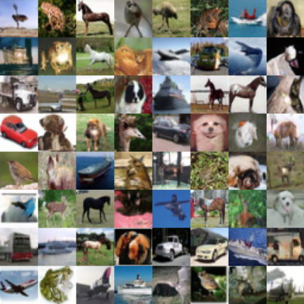
Unconditional CIFAR-10 samples from the basic DDPM model
Qualitatively the images generated by diffusion look realistic. Diffusion gets state of the art Frechet Inception Distance (FID) for CIFAR-10, which can be seen as an indicator of image quality. However it is inferior to other models with regard to the Inception Score and log-likelihood. It also gets qualitatively impressive results for other datasets like LSUN but the metrics are not the best.
Time
A significant disadvantage with diffusion is that you sample by going through each step in the making this a slow process. In this respect it is not unlike auto-regressive models where images must be generated a pixel at a time. However the image below shows that the model is starting to generate samples of decent quality well before the last step.

$\xz$ improving across timesteps
Later works show that competitive results can be obtained with fewer samples.
Extensions
A lot of work has gone into improving the limitations of diffusion models and extending its capabilities, many of which are leveraged by DALL·E 2:
- Improved Denoising Diffusion Probabilistic Models(Improved Diffusion) introduces simple modifications that improve the log likelihood.
- Diffusion Models Beat GANs on Image Synthesis manages to get better ImageNet scores compared to the best GAN models.
- Denoising Diffusion Implicit Models paper they come up with a sampling method that is able to skip some of the steps but still get good quality results.
- Whilst the model considered here, later papers suchs as Improved Diffusion also explore conditional models. It is possible to use different kinds of superivison such as labels of text inputs to generate conditional samples, a notable example is of which of course is DALL·E 2. There are different approaches to guiding diffusion models. See the GLIDE post for a discussion and references.
- Besides image generation, diffusion can be used to learn other tasks like upsampling and inpainting.
What’s next
- The appendix contains exercises that will guide you through the derivation of the loss.
- Check out this post about GLIDE to read about the conditional diffusion architecture on which DALL·E 2 is based.
- More posts on extensions to the original model coming soon.
Appendix: Loss derivation
In this section we will go through the mathematical details to understand how the approach outlined above comes about.
Terms of the loss function
As a first step we will split $L$ into three losses.
Exercise
Show that the loss $L$ may be written as
- Use Bayes rule and the Markovian property to write $\qterm$ as a product of conditional distributions $q\left(x_{t-1} \lvert x_t, x_0\right)$
- Then it is simply a question of rearranging everything and applying a little reasoning to make it match the expression
- Remember that $\DKL{q}{p} = \Eq{\log\frac{q}{p}}$
- Also recall if $a$ does not depend on $x$ then $\Ef{q(x)}{a} = a$
As both $\pr{\xT}$ and $\qrcond{\xT}{\xz}$ are fixed, $L_T = \DKL{\qrcond{\xT}{\xz}}{\pr{\xT}}$ does not depend on $\theta$ so we can neglect it from now on.
Evaluating $L_{t-1}$
To simplify $L_{t-1}$ let us consider the forward process posterior $\qrcond{\xtmone}{\xt,\xz}$. The KL-divergence is straightforward to evaluate for normal distributions. We know that the transitions in both the forward and reverse case as well as $\pr{\xtt{T}}$ are Gaussian. It turns out that the forward process posterior is also Gaussian.
Exercise
Show that $\qrcond{\xtmone}{\xt,\xz}$ is a normal distribution with mean
\[\tilde{\mu}\left(\xt, \xz \right) := \frac{\sqrt{\abtmone}\bt}{1 - \abt}\xz + \frac{\sqrt{\at}(1 - \abtmone)}{1 - \abt}\xt\]and diagonal covariance $\tbt\II$
- Remember that both $\qrcond{\xtmone}{\xz}$ and $\qrcond{\xt}{\xtmone}$ are Gaussian
- Use Bayes rule and the fact that the reverse process is Markovian to derive an expression for $\qrcond{\xtmone}{\xt, \xz}$
- Again since covariances are diagonal we need just consider the distributions for a single element
- You should be able to find an expression proportional to $\exp(-(x_{t-1} - \mu)^2/\sigma^2))$ where $x_{t-1}$ is a single element of $\xtmone$ and you can show that $\sigma^2$ and $\mu$ are equivalent to the expressions above
We have said that the reverse process transition distributions $\prtacond{\theta}{\xtmone}{\xt}$ are also Gaussian but we have not yet mentioned what form they take. Here we consider the approach from the DDPM paper where only the mean is learned whilst the covariance is set as $\sigta = \sigma_t \II$ where $\sigma_t$ is a hyperparameter. Using a diagonal covariance considerably simplifies the KL-divergence term in $L_{t-1}$.
Exercise
Show that $\def\tilmuterm{\mu\left(\xt, \xz\right)}$ $\def\thetamuterm{\mu_\theta\left(\xt, t\right)}$ \(L_{t-1} = \DKL{\qtttwo{t-1}{t}{0}}{\prtacond{\theta}{\xtmone}{\xt}}= \text{const.} + \frac{\left\Vert\tilmuterm- \thetamuterm\right\Vert^2}{2\sigma_t^2}\)
- You can use the approach in other exercises of simply considering one coordinate and then extending the answer to the multivariate case
- Neglect any constant that does not depend on
- Recall that for a Gaussian distribution $\Ef{}{x^2} = \sigma^2 + \mu^2$
Noise prediction
As mentioned above the model is trained to predict a noise value $\boldsymbol{\epsilon}_\theta(\mathbf{x}_0, t)$, from which the mean can be derived. To start with let us introduce sample $\qrcond{\xt}{\xz}$ by first sampling $\boldeps \sim \norm{\mathbf{0}, \II}$ and transforming it.
Exercise
Show that by reparameterising $\xt$ as $\xt\left(\xz, \boldeps\right) = \sqrt{\abt}\xz + \sqrt{1 - \abt}\boldeps$, $L_{t-1}$ may be written as
$\newcommand{\xtxzep}{\xt\left(\xz, \boldeps\right)}$ $\newcommand{\mutxt}{\mu_\theta\left(\xtxzep, t\right)}$
\[L_{t-1} - \text{const.} =\Ef{\xz, \boldeps}{\frac{1}{2\sigma_t^2}\left\Vert\frac{1}{\sqrt{\abt}}\left(\xtxzep - \frac{\bt}{\sqrt{1 - \abt}}\boldeps\right) -\mutxt\right\Vert^2}\]- You just need to find an expression for $\tilmuterm$ and plug it into $L_{t-1}$
To predict $\mutxt$ directly, the steps would be
- Sample $\xz \sim \qr{\xz}$, $\xt \sim \qtt{t}{0}$
- Predict $\mutxt$
However the reparameterised version of $L_{t-1}$ suggests another possibility. We see that the optimal value of $\mutxt$ is $\tilde{\mu}\left(\xt\left(\xz, \boldeps\right), \xz\right)= \muoptim$. It might be a good idea to use this form for the mean. Now the steps become
- Sample $\xz \sim \qr{\xz}$, $\boldeps \sim \norm{\mathbf{0},\II}$
- Find $\xt = \sqrt{\abt}\xz + \sqrt{1 - \abt}\boldeps$
- Predict $\etta\left(\xt, t\right)$
- Estimate $\hat{\mu} = \frac{1}{\sqrt{\abt}}\left(\xt - \frac{\bt}{\sqrt{1 - \abt}}\etta\right)$
Exercise
As it stands $L_{t-1}$ is proportional to the square difference of means $\hat{\mu}$ and $\mu_\theta$. Plugging in the expression for $\hat{\mu}$ in terms of $\etta$ and transform $L_{t-1}$ into an expression that is proportional to the squared difference of $\boldeps$ and $\etta$ up to a constant.
- Just plug in the expression for $\hat{\mu}$ and simplify
$\prtacond{\theta}{\xz}{\xtt{1}}$ as an independent discrete decoder
$L_0$ is easy to evaluate. We just need to specify what form $\prtacond{\theta}{\xz}{\xtt{1}}$ takes.
The data $\xz$ is assumed to consists of integers ${0, 1, \ldots, 255}$ linearly scaled to lie in the interval $[-1, 1]$. The form of the distribution for the last term of the reverse process is given by the products of the elementwise distributions
\(\newcommand{\deltax}[2]{\delta_{#1}\left(#2\right)}\) \(\newcommand{\deltaxzi}[1]{\deltax{#1}{x^i_0}}\) \(\def\xzi{x_0^i}\)
\[\prtacond{\theta}{\xz}{\xtt{1}} = \prod_{i=1}^D \int_{\deltaxzi{-}}^{\deltaxzi{+}} \norm{x;\mu^i_\theta\left(\xtt{1}, 1\right), \sigma_1^2} dx\] \[\deltax{+}{x}= \left\{ \begin{array}{ll} \infty & x = 1 \\ x + \frac{1}{255} & x < 1 \\ \end{array} \right.\] \[\deltax{-}{x}= \left\{ \begin{array}{ll} -\infty & x = -1 \\ x - \frac{1}{255} & x > -1 \\ \end{array} \right.\]This is more easily visualised
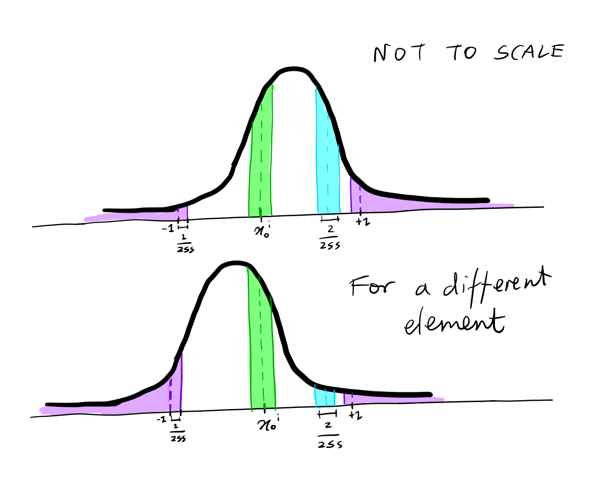
For $-1 < x < 1$, it is the interval $x-\frac{1}{255}, x+\frac{1}{255}$. For $x=1$ it is region to right of $x - \frac{1}{255}$ and for $x =-1$ it is the region to the left of $x + \frac{1}{255}$. For each element the distribution can look different as it depends on $\mu^i_\theta\left(\xtt{1}, 1\right)$. For example if the dataset contains lots of outdoor images where the sky is seen at the top of the image, blue channel elements in this region would have a high probability for $x=1$.
Exercise
Show that the expression for $\prtacond{\theta}{\xz}{\xtt{1}}$ is a valid probability distribution.
- Express the integrals for each case of $\xzi$ in terms of cumulative distribution functions $F_X(x)$
- Note that the sum over all $\xz$ may be written as product of sums over each $\xzi$
- Then you should be able to show that terms in the sum over each $\xzi$ cancel so that the result is 1
The final training objective
Whilst it is possible to use the loss directly in its simplified form, in the paper they find that the mean squared distance between the sampled noise $\boldeps$ and the predicted noise $\boldeps_\theta$ yields better sample quality
\[L_\text{simple}\left(\theta\right) := \Ef{t, \xz, \boldeps}{\left\Vert\boldeps - \etta\left(\sqrt{\abt}\xz + \sqrt{1-\abt}\boldeps\right)\right\Vert^2}\]As with a lot of things in deep learning what works in practice does not necessarily accord with theory. Nevertheless it is possible to argue that that $L_\text{simple}\left(\theta\right)$ is an approximation to the original $L$.
Exercise
Show that
- For $t>1$ that $L_\text{simple}\left(\theta\right)$ corresponds to an unweighted version of $L_{t-1}$
- For $t=1$ it is $L_0$ with the integral in $\prtacond{\theta}{\xz}{\xtt{1}}$ approximated by the probability density function of the Gaussian distribution multiplied by the bin width, neglecting edge effects and leaving out the timestep-dependent weight.
(As noted earlier $L_T$ does not depend on $\theta$ so we don’t consider it here)
- For $t>1$ you just need to identify the weights that are left out
- For $t=1$, do the approximation of the integral, then use reparameterisation of $\xtt{1}$ and $\mu_\theta$ to introduce the noise terms and eliminate the $\xtt{}$ terms and leave out the weights as for $t>1$