You have probably come across DALL-E 2 a large-scale image generation model from OpenAI. If not, you can read about it in their blog. DALL-E 2 uses a class of models known as diffusion models. The DALL-E 2 paper does not go into a lot of detail about the model architecture since it mostly extends an earlier architecture GLIDE. This article provides a brief introduction to the GLIDE architecture.
Contents
Diffusion models
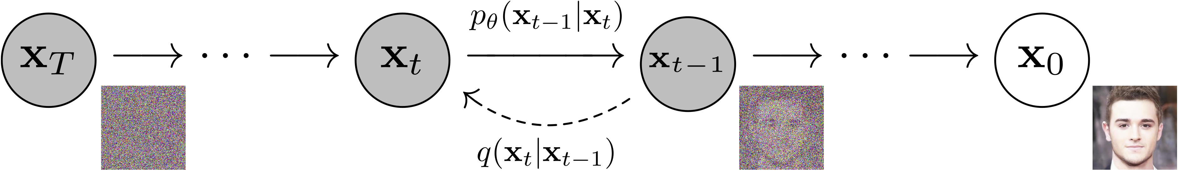
(From the DDIM paper)
Here I will quickly review diffusion models. A more in-depth tutorial on this topic is coming soon! Diffusion models assume that the data is generated through a reverse process which is a Markov chain with transitions that successively denoises a latent $\mathbf{x}_T$ until you get a sample from the data distribution $\mathbf{x}_0$
\[p\left(\mathbf{x}_T\right) = \mathcal{N}\left(\mathbf{0}, \mathbf{I}\right)\] \[p\left(\mathbf{x}_{t-1} \vert \mathbf{x}_t \right) = \mathcal{N}\left(\mu_\theta\left(\mathbf{x}_t, t\right), \Sigma_\theta\left(\mathbf{x}_t, t\right)\right)\]Associated with this forward process or diffusion process fixed to a Markov chain that successively adds more Gaussian noise to an initial data point $\mathbf{x}_0$ over a sequence of timesteps
\[q\left(\mathbf{x}_t \vert \mathbf{x}_{t-1}\right) = \mathcal{N}\left(\sqrt{1 - \beta_t}\mathbf{x}_{t-1}, \beta_t\mathbf{I}\right)\]The model learns to minimise
\[\mathbb{E}_q\left[-\log\frac{p_\theta\left(\mathbf{x}_{0:T}\right)}{q\left(\mathbf{x}_{1:T}\vert \mathbf{x}_0\right)}\right]\]which is the variational bound on the negative log likelihood
\[\mathbb{E}\left[-\log{p_\theta\left(\mathbf{x}_0\right)}\right]\]In practice you can train a model that predicts $\mu_\theta\left(\mathbf{x}_t, t\right), \Sigma_\theta\left(\mathbf{x}_t, t\right)$, and sample for $T$ successive steps from $p_\theta$ until you get to $\mathbf{x}_0$. There is also another approach which involves predicting the noise component of $\mathbf{x}_t$, $\mathbf{\epsilon}_\theta\left(\mathbf{x}_t, t\right)$ and using that to derive $\mathbf{x}_{t-1}$.
CLIP
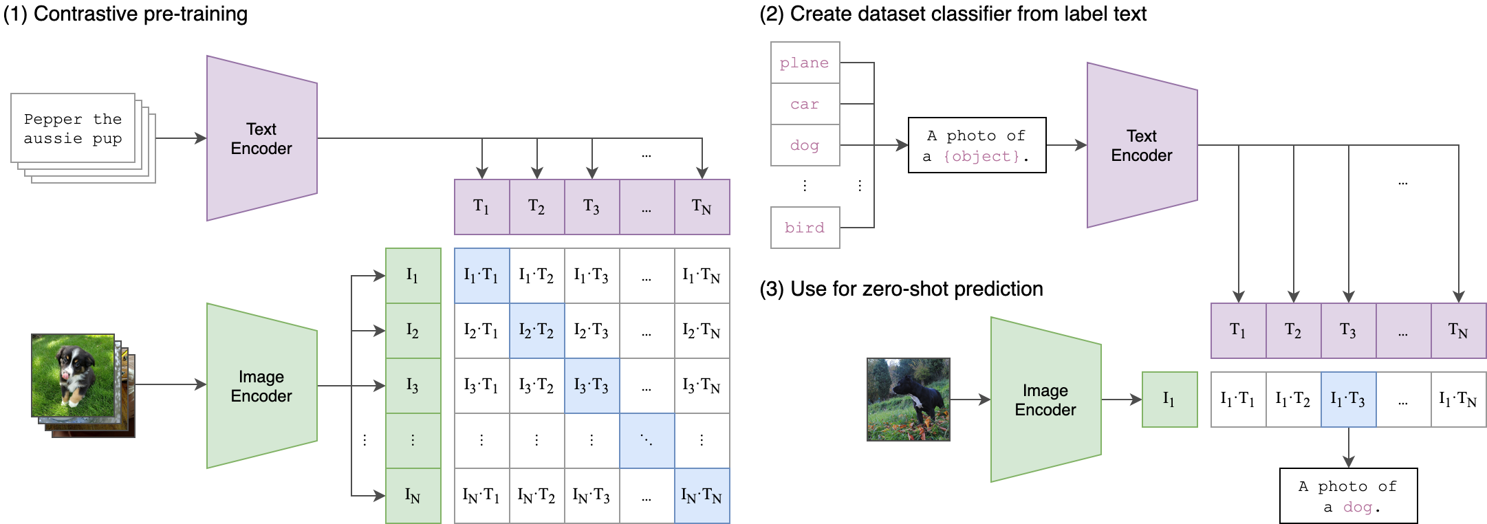
(From the CLIP paper)
OpenAI developed a large scale model jointly trained on language and image pairs using a contrastive loss. You sample pairs $(x, c)$ from a large dataset and train the model with contrastive cross-entropy loss that maximises the dot product $f(x)\cdot g(c)$ if $c$ is paired with $x$ and minimises it otherwise.
In numpy-like pseudo-code (from the CLIP paper)
# image_encoder - ResNet or Vision Transformer
# text_encoder - CBOW or Text Transformer
# I[n, h, w, c] - minibatch of aligned images
# T[n, l] - minibatch of aligned texts
# W_i[d_i, d_e] - learned proj of image to embed
# W_t[d_t, d_e] - learned proj of text to embed
# t - learned temperature parameter
# extract feature representations of each modality
I_f = image_encoder(I) #[n, d_i]
T_f = text_encoder(T) #[n, d_t]
# joint multimodal embedding [n, d_e]
I_e = l2_normalize(np.dot(I_f, W_i), axis=1)
T_e = l2_normalize(np.dot(T_f, W_t), axis=1)
# scaled pairwise cosine similarities [n, n]
logits = np.dot(I_e, T_e.T) * np.exp(t)
# symmetric loss function
labels = np.arange(n)
loss_i = cross_entropy_loss(logits, labels, axis=0)
loss_t = cross_entropy_loss(logits, labels, axis=1)
loss = (loss_i + loss_t)/2
The model can then generate embeddings for an image or a text input in a shared embedding space. That means you can find the cosine similarity of the embeddings for an image and some text, such as a caption, so that you can determine the relevance of the text to the image.
This is quite powerful because you can train zero shot classifiers by just obtaining embeddings for an image and a bunch of labels, represented as text, and predicting the one with the highest cosine similarity. In GLIDE as well as DALL-E 2, CLIP is used to supervise the generation of images.
Guided diffusion
The vanilla diffusion model generates inputs from randomly sampled latents. Later papers introduce class conditional diffusion models where a class label is also input to the model such it has mean and the variance
\[\mu_\theta\left(\mathbf{x}_t \vert y \right) \Sigma_\theta\left(\mathbf{x}_t \vert y \right)\]In addition, during sampling you can perturb prediction of the model so as to guide the sample towards the label. You can also omit the label conditioning and use the label only to guide sampling. There are several approaches to guided sampling.
Classfier-based guidance
The mean is perturbed by the gradient of the log probability of the target class $y$ predicted by a classifier.
\[\hat{\mu}_\theta\left(\mathbf{x}_t \vert y \right) = \mu_\theta\left(\mathbf{x}_t \vert y \right) + s\cdot\Sigma_\theta\left(\mathbf{x}_t \vert y \right)\nabla_{\mathbf{x}_t}\log p_\phi \left(y \vert \mathbf{x}_t \right)\]where the coefficient $s$ is called the guidance scale. The input $\mathbf{x}_t$ is from some arbitrary timestep rather than the final image. you $p_\phi$ should train one using noised images.
Classifier-free guidance
To avoid having to train an extra model, a classifier-free guidance method is proposed. Here it is assumed that the prediction of the model is $\epsilon_\theta\left(\mathbf{x}_t \vert y\right)$. You jointly train conditional and unconditional models $\epsilon_\theta\left(\mathbf{x}_t \vert y\right)$ and $\epsilon_\theta\left(\mathbf{x}_t\right)$. You can do this by randomly letting the $y$ be all zeros. Then the perturbation is then proportional to the difference between the predictions of the conditional and unconditional models.
\[\hat{\epsilon}_\theta\left(\mathbf{x}_t \right) = \epsilon_\theta\left(\mathbf{x}_t \right) + s\cdot\left(\epsilon_\theta\left(\mathbf{x}_t \vert y\right) - \epsilon_\theta\left(\mathbf{x}_t \right)\right)\]CLIP guidance
As mentioned earlier, CLIP comprises two parts, an image encoder $f(x)$ and a caption encoder $g(c)$. This approach is similar to guided diffusion except that the perturbation is the dot product of $g(c)$ and $f(\mathbf{x}_t)$
\[\hat{\mu}_\theta\left(\mathbf{x}_t \vert c \right) = \mu_\theta\left(\mathbf{x}_t \vert c \right) + s\cdot\Sigma_\theta\left(\mathbf{x}_t \vert c \right)\nabla_{\mathbf{x}_t}\log\left(f(\mathbf{x}_t)\cdot g(c)\right)\]Similar to classifier based guidance, they train the CLIP model with noised images.
GLIDE
GLIDE use a conditional version the original diffusion architecture and replaces the label input with text conditioning information. The model generates samples from $p\left(\mathbf{x}_t \vert \mathbf{x}_{t-1}, c\right)$.
The architecture is a U-Net type model with a combination of residual blocks of convolutional layers and attention blocks.
The inputs comprise a caption $c$, an image $\mathbf{x}_t$ and a timestep $t$. The timestep is transformed to a harmonic embedding and then projected via linear layers
emb = self.time_embed(timestep_embedding(timesteps, self.model_channels))
It can be added to the output of the residual block.
The text input is processed as follows
- Encode $c$ into a sequence of $K$ tokens
- Feed this into a Transformer model
In code, from the official implementation
xf_in = self.token_embedding(tokens.long())
xf_in = xf_in + self.positional_embedding[None]
if self.xf_padding:
    assert mask is not None
    xf_in = th.where(mask[..., None], xf_in, self.padding_embedding[None])
xf_out = self.transformer(xf_in.to(self.dtype))
if self.final_ln is not None:
    xf_out = self.final_ln(xf_out)
xf_proj = self.transformer_proj(xf_out[:, -1])
xf_out = xf_out.permute(0, 2, 1)  # NLC -> NCL
The final token embedding x_proj is used in place of a class embedding and added to the timestep embedding
text_outputs = self.get_text_emb(tokens, mask)
xf_proj, xf_out = text_outputs["xf_proj"], text_outputs["xf_out"]
emb = emb + xf_proj.to(emb)
In addition, the last layer of K token embeddings, x_out are input to each attention layer of the U-Net model by projecting (encoder_kv), then concatenating to the key and value attention inputs
ek, ev = encoder_kv.reshape(bs * self.n_heads, ch * 2, -1).split(ch, dim=1)
k = th.cat([ek, k], dim=-1)
v = th.cat([ev, v], dim=-1)
The model outputs 64 x 64 images so they train an upsampling model also conditioned on text inputs to generate final outputs of size 256 x 256.
In the paper they experiment with classifier-free and CLIP-based guidance. To support classifier-free guidance they fine-tune the model whilst replacing 20% of the captions with an empty sequence. This way the model can generate both text-conditioned and unconditional outputs.
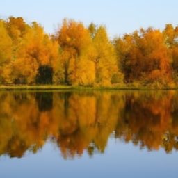
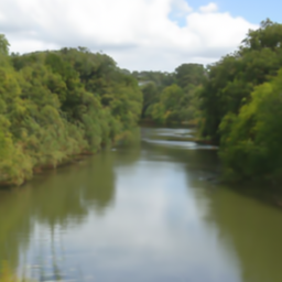
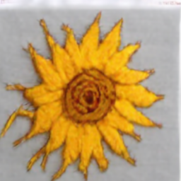
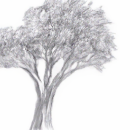
Examples
The model is able to generate diverse inputs. OpenAI has not released the full model on the basis that it could potentially be used to generate harmful images. However they have released a smaller variant and I tried to see how well it demonstrated the capabilities of the full-sized model. You can try out the model via the Colab notebooks here.
In general it was not so good at responding to prompts as complex as in the examples in the paper and did not always match perfectly with the caption. Please see the paper for examples from the full-sized model. To generate the example, I kept trying until I got a reasonable result.
The capabilities in the paper mentioned include the ability to
- Generate realistic-looking images with shadows, textures and reflections
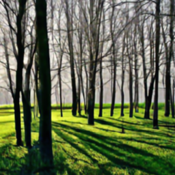
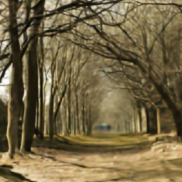
- Generate images in different styles and different media
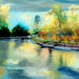
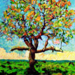
- Compose different concepts and bind attributes to objects for example colours. The small model seems to find this more difficult and I have included failure cases.
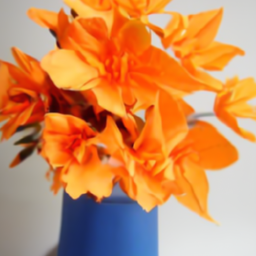
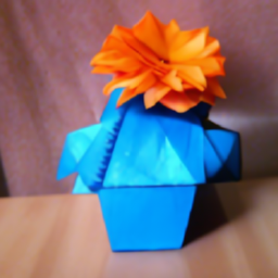
- Examples using prompts from the paper where the small model produces inferior results (I tried about 5-10 times)
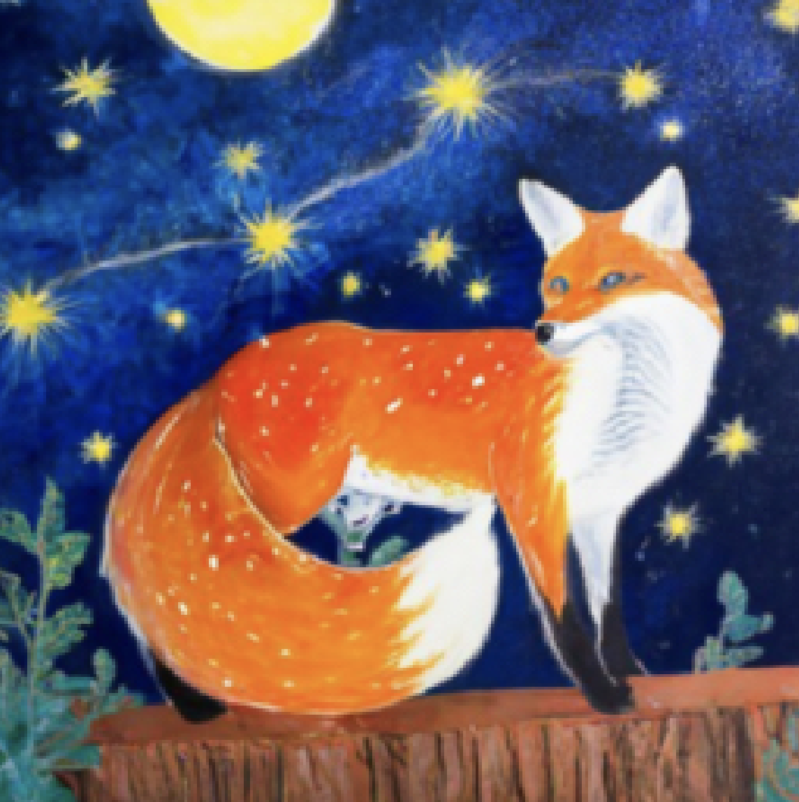
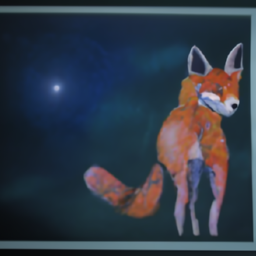
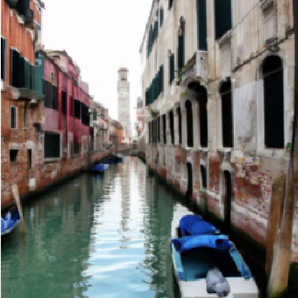
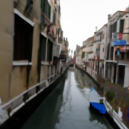
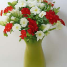
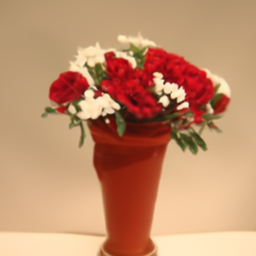
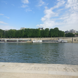
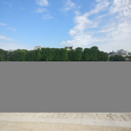
Image editing
As the name of the model implies, it is possible to use it to make changes to an image. For this they fine-tune the model by feeding in images with random regions erased. Their model is capable of making realistic edits, adding objects, shadows and reflections. I encourage you to refer to the paper for high-quality examples of in-painting which includes multi-stage image editing. But just for fun I generated a couple of examples using the small model.
Results
- Classifier-free guidance leads better Precision/Recall and Inception score/Fréchet Inception distance trade-off.
- CLIP guidance leads perhaps not unsurprisingly to a better CLIP score/FID tradeoff on MS-COCO but humans find the samples using classifier-free guidance to be more photo-realistic and in better agreement with text prompts.
- Humans also find GLIDE samples to be more photo-realistic and in better agreement with the captions compared to those from DALL-E even though the latter also uses CLIP to re-rank the images.
- The model’s zero-shot FID score on the MS-COCO dataset is better than several models that were trained on this dataset (although higher than the best performing models).
Summary
- GLIDE is a diffusion-based image generation model that is conditioned on text prompts.
- The model comprises an initial network generates a 64 x 64 image and a further upsampling network that produces a 256 x 256 image.
- It is also capable of image in-painting.
- Sample generation can be guided using CLIP or in a classifier-free manner where classifier-free guidance leads to samples that are preferred by humans.
- Humans also prefer the samples from GLIDE to those from DALL-E.
- The model gets competitive zero-shot MS-COCO FID.
References
- GLIDE: Towards Photorealistic Image Generation and Editing with Text-Guided Diffusion Models (link)
- Learning Transferable Visual Models From Natural Language Supervision (CLIP paper) (link)
- Denoising Diffusion Probabilistic Models (DDIM paper) (link)
- Diffusion Models Beat GANs on Image Synthesis (classifier-based guided diffusion) (link)
- Classifier-Free Diffusion Guidance (link)