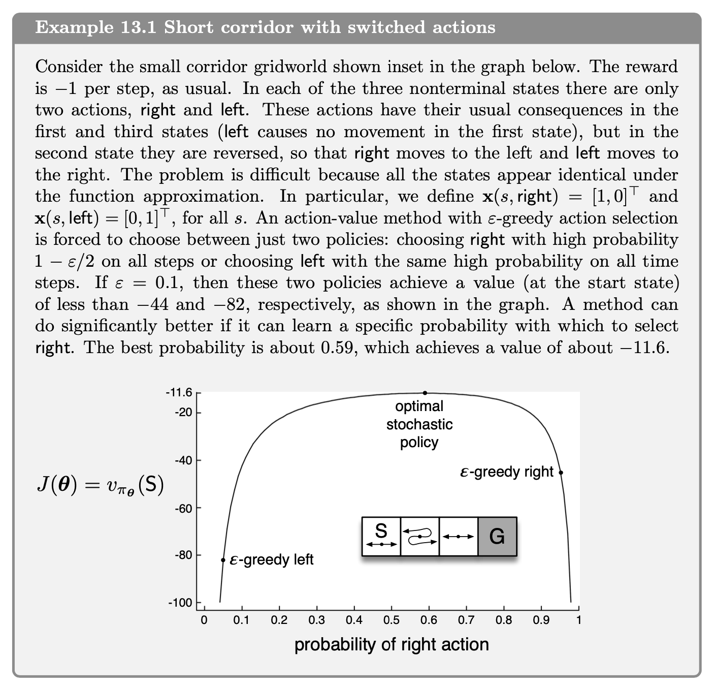
In this tutorial we will demonstrate how to implement Example 13.1 of Reinforcement Learning (Sutton and Barto). You can read more about this algorithm in the book. Here is the task description
I highly encourage you to study the chapter on your own and try to implement the example by yourself, referring to this post as needed.
Deriving the probability of the right action
Let $\pi(R \vert s) = p, \pi(L \vert s) = (1 - p)$ for all states $s$ and let $R$ and $L$ denote actions right and left. Then the state values are as follows
- For $s=1$ ($S$ in the figure), since $L$ makes it stay in the same state.
- For $s=2$, since from this state you move in the opposite direction as $a$
- For $s=3$, since $R$ goes to a terminal state with value of 0
This gives rise to the following system of equations that can be solved for the values $v_\pi\left(S\right)$.
\(p\cdot v_\pi(2) - p\cdot v_\pi(1) = 1\) \((1-p)\cdot v_\pi(3) + v_\pi(2) - p\cdot v_\pi(1) = 1\) \(-p\cdot v_\pi(3) + (1-p)\cdot v_\pi(2) = 1\)
Then as in the example we solve for $p$ as the probability that maximises the value of $v_\pi\left(1\right)$.
Solving for the probability of the right action
We will write the equations above in matrix form to make it easy to solve. We will be using a python library called sympy for this purpose. Don’t worry if you have not used it before. The code below is quite straightforward to follow and will introduce you to some features of the library.
import sympy as sy

# Create a symbol
p = sy.Symbol('p')

# Create a matrix
A =sy.Matrix([
    [-p, p, 0],
    [p,-1,(1-p)],
    [0,(1-p),-1]
])

# Create a vector
b = sy.Matrix([[1], [1], [1]])
Solve $A\mathbf{v} = b$
v = sy.simplify(A.inv() @ b)
Now we can find $p$ that maximises $v_\pi(S) = v_\pi(1)$
v[0]
$\displaystyle \frac{2 \cdot \left(2 - p\right)}{p \left(p - 1\right)}$
sols = sy.solve(v[0].diff(p))
# Convert to float
list(map(float, sols))
[0.585786437626905, 3.414213562373095]
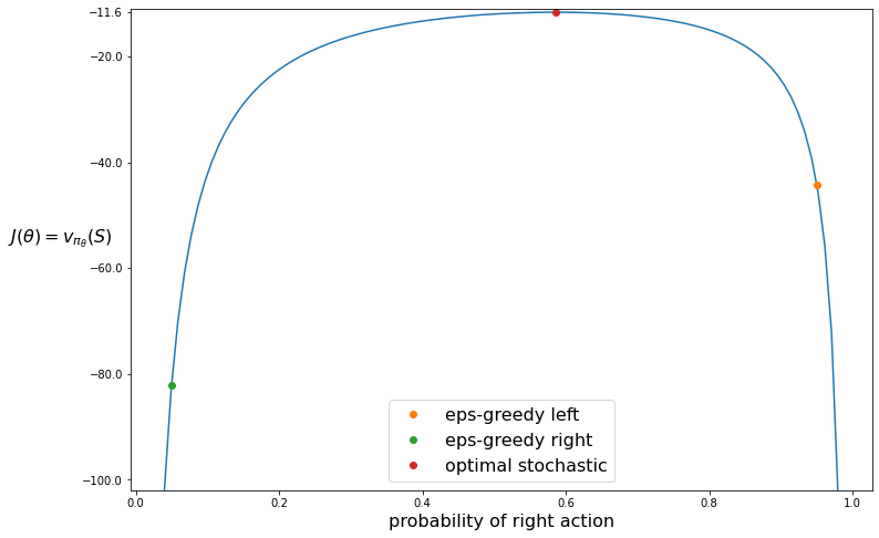
Creating the plot
Compare this value with the $\epsilon$-greedy right and left values where $\epsilon=0.1$
# The first value is the valid one for the probability as it is in the interval [0, 1]
p_best = sols[0]
eps = 0.1
v_eps_r, v_best, v_eps_l = float(v[0].subs(p, 1-eps/2)), float(v[0].subs(p, p_best)), float(v[0].subs(p, eps/2))

print('eps-greedy left: {:.2f}, optimal stochastic: {:.2f}, eps-greedy-right: {:.2f}'.format(v_eps_r, v_best, v_eps_l))
eps-greedy left: -44.21, optimal stochastic: -11.66, eps-greedy-right: -82.11
import matplotlib.pyplot as plt
import numpy as np
probs = np.linspace(0.04, 0.98, 101)
vals = [v[0].subs(p, i) for i in probs]
plt.figure(figsize=(12, 8))
plt.plot(probs, vals)
plt.plot(1-eps/2, v_eps_r, linewidth=0, marker='o', label='eps-greedy left');
plt.plot(eps/2, v_eps_l, linewidth=0,marker='o', label='eps-greedy right');
plt.plot(p_best, v_best, linewidth=0, marker='o', label='optimal stochastic');
plt.xlabel('probability of right action', fontsize=16)
plt.ylabel('$J(\\theta) = v_{\pi_{\\theta}}(S)$\t',fontsize=16, rotation=360)
plt.legend(fontsize=16);

yticks = plt.yticks()
plt.yticks(np.concatenate([yticks[0], [-11.6]]));
plt.ylim(-102, -11);
Summary
In this article we showed how to recreate Example 13.1 from Sutton and Barto. In a subsequent post we will implement the REINFORCE algorithm to tackle this task.