\(\newcommand{\vv}{\mathbf{v}}\) In machine learning applications you sometimes want to interpolate vectors in a normalised latent space such as when interpolating between two images in a generative model. An appropriate method for doing this is spherical interpolation. In this post we will derive the formula for this method and show how it differs from linear interpolation.
Linear Interpolation
You are probably know how to do linearly interpolation. It can be characterised as a function $\text{lerp}(\mathbf{v}_1, \mathbf{v}_2, t)$. There are two vectors $\mathbf{v}_1$ and $\mathbf{v}_2$ and a weight $t$ which indicates how much to weight $\mathbf{v}_2$ whilst $\mathbf{v}_1$ is weighted by $(1 - t)$
\[\text{lerp}(\mathbf{v}_1, \mathbf{v}_2, t) = (1 - t)\mathbf{v}_1 + t\mathbf{v}_2\]Let us look at a simple example in two dimensions.
import numpy as np
import matplotlib.pyplot as plt
v1 = np.stack([np.cos(5*np.pi/12), np.sin(5*np.pi/12)])
v2 = np.stack([np.cos(np.pi/12), np.sin(np.pi/12)])
plt.figure(figsize=(8, 8))
plt.arrow(0, 0, *v1, color='cornflowerblue', linewidth=3, head_width=0.02, label='v1', length_includes_head=True)
plt.text(0.08, 0.6, '$v_1$', color='cornflowerblue', fontsize=16)
plt.arrow(0, 0, *v2, color='seagreen', linewidth=3,  head_width=0.02, label='v2', length_includes_head=True)
plt.text(0.6, 0.2, '$v_2$', color='seagreen', fontsize=16)
t = 0.75
v = (v1 * (1 - t) + v2 * t)


plt.hlines(xmin=0, xmax=v[0], y=v[1], linestyle='--', color='indigo', alpha=0.6)
plt.vlines(ymin=0, ymax=v[1], x=v[0],  linestyle='--', color='purple', alpha=0.6)
plt.xticks([0, 0.5, v[0], 1.])
plt.gca().set_xticklabels([0, 0.5, f'x1*(1-t) + x2*t = {v[0]:.2f}', 1.], fontsize=12)
plt.yticks([0, v[1], 0.5, 1.])
plt.gca().set_yticklabels([0, f'y1*(1-t) + y2*t = {v[1]:.2f}', 0.5, 1.], fontsize=12)
plt.arrow(0, 0, *v, color='turquoise', linewidth=3,  head_width=0.02, label='v', length_includes_head=True)
plt.text(0.35, 0.25, '$v$', color='turquoise', fontsize=16)
plt.plot([v[0], v2[0]], [v[1], v2[1]], color='red', alpha=0.5, linestyle='--',)
plt.text(0.9, 0.35, '(1-t)|v1 - v2| = 0.25', color='red', fontsize=12, backgroundcolor='white')
plt.plot([v[0], v1[0]], [v[1], v1[1]], color='darkorange', alpha=0.5, linestyle='--',)
plt.text(0.6, 0.65, 't|v1 - v2| = 0.75', color='darkorange', fontsize=12)
plt.xlim([0, 1])

plt.ylim([0, 1]);
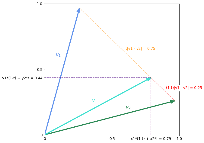
As the figure shows we interpolate in every direction. Equivalently we can think of it as moving a fraction $t$ of the the way along the straight line joining $\mathbf{v}_1$ and $\mathbf{v}_2$. The following relations hold for the distance between $\mathbf{v}$ and the endpoints
\[\vert \vv - \vv_1 \vert = t\vert \vv_2 - \vv_1 \vert\] \[\vert \vv - \vv_2 \vert = (1 - t)\vert \vv_2 - \vv_1 \vert\]An issue with linear interpolation is that even when the endpoint vectors are normalised, interpolated vector is not. In the figure above you can see that $\mathbf{v}$ is smaller than $\mathbf{v}_1$ and $\mathbf{v}_2$ both of which are normalised. When interpolating vectors in a normalised latent space you want to sample points on a hypersphere. The appropriate method for this is spherical interpolation.
Spherical interpolation
plt.figure(figsize=(8, 8))
plt.arrow(0, 0, *v1, color='cornflowerblue', linewidth=3, head_width=0.02, label='v1', length_includes_head=True)
plt.text(0.08, 0.6, '$v_1$', color='cornflowerblue', fontsize=16)
plt.arrow(0, 0, *v2, color='seagreen', linewidth=3,  head_width=0.02, label='v2', length_includes_head=True)
plt.text(0.6, 0.2, '$v_2$', color='seagreen', fontsize=16)

dtheta = np.pi / 100
theta = np.arange(np.pi/12, 5*np.pi/12, dtheta)
x = np.cos(theta)
y = np.sin(theta)
plt.plot(x * 0.2,y * 0.2, color='indigo')
plt.text(0.15, 0.15, '$\Omega$', color='indigo', fontsize=16);

theta_full = np.arange(0, np.pi/2 + dtheta, dtheta)
plt.plot(np.cos(theta_full),np.sin(theta_full), color='maroon')
plt.xlim([0, 1])

plt.ylim([0, 1]);
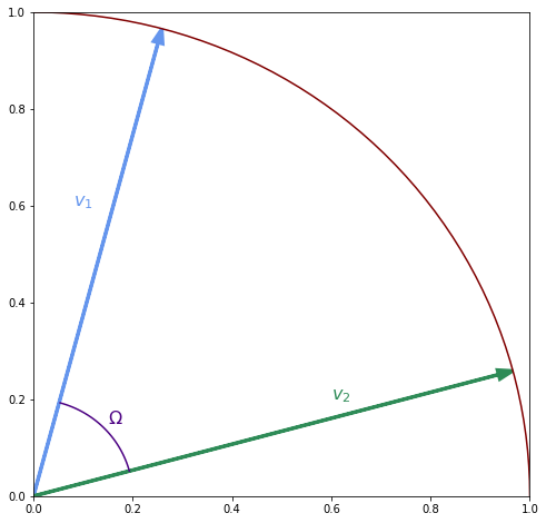
Since we are assuming that the two vectors are normalised you can think of them as points on the surface of a unit sphere. In 2d that the “sphere” is just a circle as show in the figure above. This time to interpolate you rotate between the vectors. In spherical interpolation a similar kind of relationship exists for the angles between the vectors as for the distances in linear interpolation. Let $\Omega$ denote the angle between $\vv_1$ and $\vv_2$, let $\theta_1$ denote the angle between $\vv$ and $\vv_1$ and $\theta_2$ the angle between $\vv_1$ and $\vv_2$. Then we have
\[\theta_1 = t\Omega\] \[\theta_2 = (1 - t)\Omega\]Since the vectors are assumed to be normalised
\[\Omega = \cos^{-1}\left(\mathbf{v}_1 \cdot \mathbf{v}_2\right)\]The interpolated vector $\vv$ should be such that
\[\vv\cdot\vv_1 = \cos\theta_1 = \cos \left({t\Omega}\right)\] \[\vv\cdot\vv_2 = \cos\theta_2 = \cos \left({(1 - t)\Omega}\right)\]The vector can be written as
\[\vv = \alpha \vv_1 + \beta \vv_2\]To derive $\alpha$ and $\beta$, take the dot product with $\vv_1$ and $\vv_2$ and substitute the equations above and solve the simultaneous equations
\[\vv \cdot \vv_1 = \alpha + \beta\cos\Omega = \cos \left({t\Omega}\right)\] \[\vv \cdot \vv_2 = \alpha\cos\Omega + \beta = \cos \left({(1- t)\Omega}\right)\]Multiply the first equation by $\cos(\Omega)$, subtract from the second and solve for $\beta$
\[\beta(1 - \cos^2\Omega) = \beta\sin^2\Omega = \cos \left({(1- t)\Omega}\right) - \cos \left({t\Omega}\right)\cos\Omega\] \[=\cos\left(t\Omega\right)\cos\left(\Omega\right) + \sin\left(t\Omega\right)\sin\left(\Omega\right) - \cos \left({t\Omega}\right)\cos\Omega = \sin\left(t\Omega\right)\sin\Omega \\ \implies \beta = \frac{\sin\left(t\Omega\right)}{\sin\Omega}\]Plug this into the first equation, multiply through by $\sin\Omega$ and rearrange to solve for $\alpha$
\[\alpha\sin\Omega = \sin\Omega \cos \left({t\Omega}\right)- \cos\Omega\sin\left(t\Omega\right) = \sin((1 - t)\Omega) \\ \implies \alpha = \frac{\sin\left((1 - t)\Omega\right)}{\sin\Omega}\]In summary
\[\text{slerp}(\mathbf{v}_1, \mathbf{v}_2, t) = \frac{\sin\left((1 - t)\Omega\right)}{\sin\Omega}\mathbf{v}_1 + \frac{\sin\left(t\Omega\right)}{\sin\Omega}\mathbf{v}_2\]As an exercise take the dot product of this with $\vv_1$ and $\vv_2$ and ensure that you get the values expected.
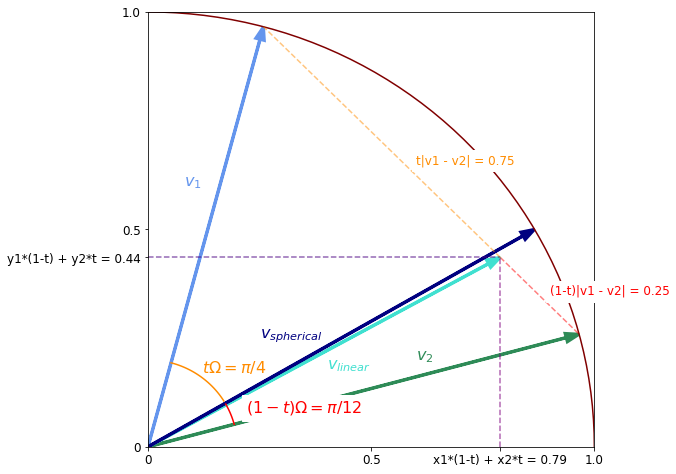
Finally we can put everything together to compare the two types of interpolation.
plt.figure(figsize=(8, 8))
plt.arrow(0, 0, *v1, color='cornflowerblue', linewidth=3, head_width=0.02, label='v1', length_includes_head=True)
plt.text(0.08, 0.6, '$v_1$', color='cornflowerblue', fontsize=16)
plt.arrow(0, 0, *v2, color='seagreen', linewidth=3,  head_width=0.02, label='v2', length_includes_head=True)
plt.text(0.6, 0.2, '$v_2$', color='seagreen', fontsize=16)

theta_full = np.arange(0, np.pi/2 + dtheta, dtheta)
plt.plot(np.cos(theta_full),np.sin(theta_full), color='maroon')

Omega = np.pi / 3 # = 5pi/12 - pi/12

assert np.isclose(np.arccos((v1*v2).sum(-1)), Omega)

v_spherical = (v1 * np.sin((1 - t)*Omega) + v2 * np.sin(t*Omega)) / np.sin(Omega)

plt.hlines(xmin=0, xmax=v[0], y=v[1], linestyle='--', color='indigo', alpha=0.6)
plt.vlines(ymin=0, ymax=v[1], x=v[0],  linestyle='--', color='purple', alpha=0.6)
plt.xticks([0, 0.5, v[0], 1.])
plt.gca().set_xticklabels([0, 0.5, f'x1*(1-t) + x2*t = {v[0]:.2f}', 1.], fontsize=12)
plt.yticks([0, v[1], 0.5, 1.])
plt.gca().set_yticklabels([0, f'y1*(1-t) + y2*t = {v[1]:.2f}', 0.5, 1.], fontsize=12)
plt.arrow(0, 0, *v, color='turquoise', linewidth=3,  head_width=0.02, label='v', length_includes_head=True)
plt.text(0.4, 0.18, '$v_{linear}$', color='turquoise', fontsize=16)
plt.plot([v[0], v2[0]], [v[1], v2[1]], color='red', alpha=0.5, linestyle='--',)
plt.text(0.9, 0.35, '(1-t)|v1 - v2| = 0.25', color='red', fontsize=12, backgroundcolor='white')
plt.plot([v[0], v1[0]], [v[1], v1[1]], color='darkorange', alpha=0.5, linestyle='--',)
plt.text(0.6, 0.65, 't|v1 - v2| = 0.75', color='darkorange', fontsize=12, backgroundcolor='white');

plt.arrow(0, 0, *v_spherical, color='navy', linewidth=3,  head_width=0.02, label='v', length_includes_head=True)
plt.text(0.25, 0.25, '$v_{spherical}$', color='navy', fontsize=16)

dtheta = np.pi / 100
theta1 = np.arange(5*np.pi/12, 5*np.pi/12 - t*Omega, -dtheta)
theta2 = np.arange(np.pi/12, np.pi/12 + (1 - t)*Omega, dtheta)
x1 = np.cos(theta1)
y1 = np.sin(theta1)
plt.plot(x1 * 0.2,y1 * 0.2, color='darkorange')
plt.text(0.12, 0.17, '$t\Omega = \pi/4$', color='darkorange', fontsize=16);

x2 = np.cos(theta2)
y2 = np.sin(theta2)
plt.plot(x2 * 0.2,y2 * 0.2, color='red')
plt.text(0.22, 0.08, '$(1-t)\Omega = \pi/12$', color='red', fontsize=16, backgroundcolor='white');


plt.xlim([0, 1])
plt.ylim([0, 1]);