You might have encountered the term importance sampling in a machine learning paper. This post provides a quick hands-on introduction to this topic. Hopefully after reading it you will have know understand how to use this technique in practice.
A quick review of sample averages
Let $x \sim f(x)$ be a continuous random variable. The expected value of $x$ is
\[E_{x\sim f}\left[x\right] = \int x f(x) dx\]More generally the expected value of any function $h(x)$ is
\[E_{x\sim f}\left[h(x)\right] = \int h(x) f(x) dx\]Sometimes such as when $f(x)$ is the Gaussian distribution this integral can be evaluated exactly. But when this is not possible you can approximate using sample averages. Take $N$ samples $x_i \sim f(x)$ and approximate the integral by a the mean of these samples
\[E_{x\sim f}\left[h(x)\right] \approx \frac{1}{N}\sum_{x_i \sim f}h(x_i)\]By the law of large numbers as $N \rightarrow \infty$ this approaches the exact expected value.
\[E_{x\sim f}\left[h(x)\right] = \int h(x) f(x) dx = \lim_{N \rightarrow \infty}\frac{1}{N}\sum_{x_i \sim f} h(x_i)\]As an example consider $h(x) = x^2$ and $f(x) = \mathcal{N}(0, 1)$. Here we know for a fact that $E[x^2] = 1$.
import numpy as np
import matplotlib.pyplot as plt
from scipy.stats import norm
plt.figure(figsize=(8, 4))
N = np.logspace(1, 4, 21).astype('int')
E_xsq = []
for Ni in N:
    samples = np.random.normal(size=[Ni])
    E_xsq.append((samples**2).mean())

plt.semilogx(N, np.abs(np.subtract(1, E_xsq)), marker='x')
plt.title('$|1 - (1/N)\sum_{x_i \sim f}{x_i^2}|$ for different values of $N$');
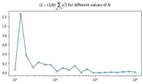
We can see that as $N$ increases the error $\left\vert1 - (1/N)\sum_{x_i \sim f}{x_i^2}\right\vert$ decreases. Now we shall plot a histogram of 1000 estimates for $N = 100, 1000, 10000$.
plt.figure(figsize=(8, 4))
for Ni in [100, 1000, 10000]:
    samples = np.random.normal(size=[Ni, 1000])
    plt.hist((samples**2).mean(0), alpha=0.5, bins=100, label=f'N={Ni}');

plt.legend();
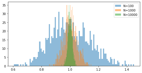
Note that as $N$ increases the histogram becomes narrower indicating that there is is less variance in the estimates.
The need for importance sampling
The sample average estimate is simple and frequently used. The loss function in training neural networks is often a sample average, for example the softmax cross-entropy loss, where $y$ is a onehot vector
\[L_\text{BCE} = E_{(x, y) \sim p_\text{data}}\left[-y^T\log h_\theta\left(x\right)\right] \approx -\frac{1}{N}\sum_{(x_i, y_i) \sim p_\text{data}}y_i^T\log h_\theta\left(x_i\right)\]However there are some potential issues
- It might be hard to sample from $f(x)$
- The samples might not be informative - for example the overlap between the support of $f(x)$ and the domain of $h(x)$ is small.
In this post we will focus on the second issue. Previously we saw that as the number of samples $N$ increased the variance of the estimate decreased. We might ask if we by having more informative samples we could reduce the variance without increasing the number of samples.
In importance sampling we find another distribution or a “proposal” distribution $q(x)$ and to turn $E_{x\sim f}\left[h(x)\right]$ into an expectation over $q$
\[E_{x\sim f}\left[h(x)\right] = \int h(x) f(x) dx = \int h(x) f(x) \frac{q(x)}{q(x)} dx = \int h(x) \frac{f(x)}{q(x)} q(x)dx = E_{x\sim q}\left[h(x) \frac{f(x)}{q(x)} \right]\]Now we can approximate $E_{x\sim q}\left[f(x) \frac{p(x)}{q(x)} \right]$ as before
\[E_{x\sim p}\left[f(x)\right] = E_{x\sim q}\left[f(x) \frac{p(x)}{q(x)} \right] \approx \frac{1}{N}\sum_{i=1}^N f(x_i)\frac{p(x_i)}{q(x_i)} = \frac{1}{N}\sum_{i=1}^N f(x_i)w(x_i)\]where the samples are weighted by $w(x_i)$. If $x_i$ is equally likely according to $q$ as well as $p$ then the sample is treated the same way as in the earlier approximation. If it is less likely according to $p$ relative to $q$ it is scaled down but this will be offset by the fact that you will have more samples from $q$ with a high probability.
Importance sampling example
Consider the integral
\[\int_0^\pi x \sin x \cdot dx\]We know how to integrate this and the answer is in fact
\[\left.x\sin x \right\vert_0^\pi = \pi\]This can be written in terms of an expectation over $x \sim U(0, \pi)$
\[\int_0^\pi x \sin x \cdot dx = \pi\int_0^\pi \frac{1}{\pi} x \sin x \cdot dx = \pi E_{x \sim U(0, \pi)}\left[x \sin x\right]\]Let us take a look at the function
plt.figure(figsize=(8, 4))
hx = lambda x: x*np.sin(x)

xmin = 0
xmax = np.pi

x = np.linspace(xmin, xmax, 1000)

plt.plot(x, hx(x), label='$x\sin x$');
plt.hlines(xmin=xmin, xmax=xmax, y=1/xmax, label='$1/\pi$', color='k');
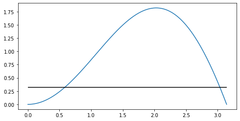
Here you can see that the peak of the function around $x=2$ will contribute most to the integral and the values close to the endpoints much less. However if you sample from $f(x) = U(0, \pi)$ you would sample equally from the whole interval $[0, \pi]$. We would like to sample more points from round the peak.
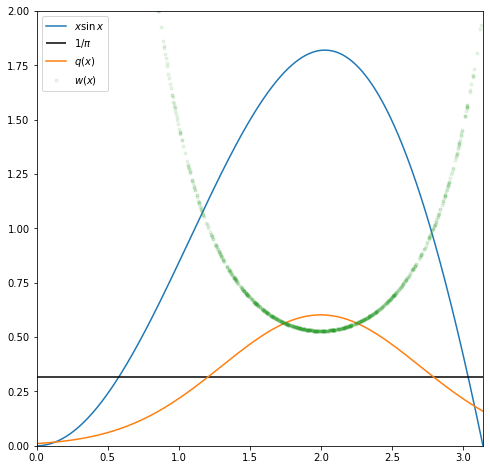
Since $x\sin x$ looks roughly like a Gaussian with a peak round $x=2$ let us try using as a proposal $N(2, 0.7)$ after scaling it so that its support is the same as the domain of $h(x)$ i.e. $\left[0, \pi\right]$.
plt.figure(figsize=(8, 8))
mu = 2
sigma = .7
n_samples = 1000
n_estimates = 1000
normal = norm(loc=mu, scale=sigma)
# Scale so that it covers the same domain as h(x)
denom = normal.cdf(xmax) - normal.cdf(xmin)
qx = lambda x: normal.pdf(x) / denom
wx = lambda x: (1/xmax) / qx(x)


xmin = 0
xmax = np.pi

x = np.linspace(xmin, xmax, n_samples)


plt.plot(x, hx(x), label='$x\sin x$');
plt.hlines(xmin=xmin, xmax=xmax, y=1/xmax, label='$1/\pi$', color='k');
plt.plot(x, qx(x), label='$q(x)$');

samples = np.random.normal(loc=mu, scale=sigma, size=n_samples);
plt.plot(samples, wx(samples), '.', label='$w(x)$', alpha=0.1);
plt.ylim(0, 2);
plt.xlim(xmin, xmax);
plt.legend();
First take samples from $f(x)$ and find estimates.
uniform_estimates = np.stack([
    hx(np.random.uniform(xmin, xmax, size=[n_samples])).mean() * np.pi
    for i in range(n_estimates)
])
Now do importance sampling. Here we need to be a bit careful since we want to restrict samples to the domain of $h(x)$ so we retain only those samples are in this domain.
is_estimates = []
num_rejected = []
for i in range(n_estimates):
    n_samples_left = n_samples
    samples = []
    n = 0
    while n_samples_left > 0:
        s = np.random.normal(loc=mu, scale=sigma, size=n_samples_left)
        s = s[(s<xmax) & (s>xmin)]
        n += (n_samples_left - len(s))
        samples = np.concatenate([samples, s])
        n_samples_left -= len(s)

    num_rejected.append(n)
    is_estimates.append(
        (hx(samples) * wx(samples)).mean() * np.pi
    )
Out of interest the number of rejected samples is small relative to total number of samples
np.mean(num_rejected / np.add(n_samples, num_rejected))
0.053700062413939764
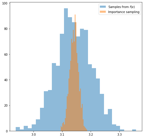
Comparing the histograms for the two sets of estimates we can see that the variance is much smaller when we using importance sampling.
plt.figure(figsize=(8, 8))
plt.hist(uniform_estimates, bins=30, alpha=0.5, label='Samples from $f(x)$');
plt.hist(is_estimates, bins=30, alpha=0.5, label='Importance sampling');
plt.legend();
print("Exact solution: ", np.pi)
print("Mean of estimates using x ~ f(x): ", np.mean(uniform_estimates))
print("Standard deviation of estimates using x ~ f(x) ", np.std(uniform_estimates))
print("Mean of estimates using importance sampling: ", np.mean(is_estimates))
print("Standard deviation of estimates using importance sampling: ", np.std(is_estimates))
Exact solution:  3.141592653589793
Mean of estimates using x ~ f(x):  3.1405385491946087
Standard deviation of estimates using x ~ f(x)  0.06185643911655511
Mean of estimates using importance sampling:  3.1414545418966644
Standard deviation of estimates using importance sampling:  0.015353005384556133
References
- The importance sampling example is borrowed from the lecture 4 of Harvard’s AM207: Stochastic Optimisation which was run in 2017. The codebase and resources for this course can be found here.