Introduction
In this post we will implement Example 9.1 from Chapter 9 Reinforcement Learning (Sutton and Barto). This is an example of on-policy prediction with approximation which means that you try to approximate the value function for the policy you are following right now. We will be using Gradient Monte Carlo for approximating $v_\pi(s)$
I strongly suggest that you study sections 9.1-9.3 of this chapter (as well as first 4 chapters of the book if you are not familiar with RL) and that you have a go at implementing the example yourself using this blogpost as a reference in case you get stuck. You can also take a look at this post involving ideas from the earlier chapters.
Task description
From page 202 of the text
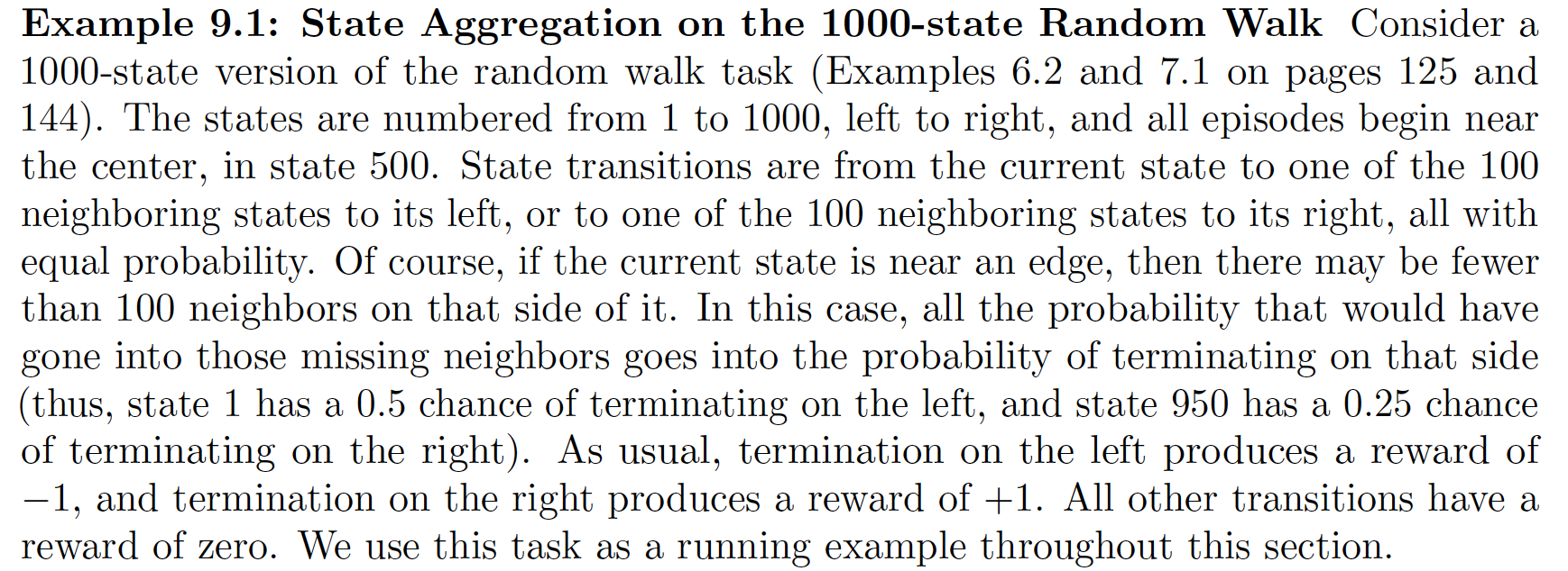
Task breakdown
- Left terminal state L, right terminal state R
- $s, a \in [1, 1000] \cup {L, R}$
- Neighbours $N_s = {x: 0 < \lvert x - s \rvert \leq 200}$
- For $a \in [1, 1000]$:
- For the terminal actions
- Transitions and rewards are deterministic given $(s, a)$ \(s' = a\) \(r = \begin{cases} 1 & a = R \\ -1 & a = L \\ 0 & \text{otherwise} \end{cases}\)
Exact solution for $v_\pi(s)$
Now let us write down the value function for the different cases which will give us a system of equations that can be solved to get the true value. Note that here we do not explicitly include $L$ and $R$ which we defined for convenience. Their values are equal to $0$ and plugging those in gives a system of 1000 equations with 1000 unknowns.
\[v_\pi(s) = \sum_a \pi(a\vert s) \sum_{s'}\sum_r p(s', r \vert s, a)\left[r + \gamma v_\pi(s')\right]\]- $100 < s \leq 900$, remembering that for all transiations to non-terminal states $r=0$
- $s \leq 100$, since for transition to $L$, $r=-1$ and value of terminal state is $0$
- $s > 900$, since for transition to $R$, $r=1$ and value of terminal state is $0$
Concisely we can write
\[v_\pi(s) - \frac{1}{200}\sum_{s' \in N_s}v_\pi(s') = -\mathbb{1}_{s \leq 100} + \mathbb{1}_{s > 100} ,\text{ } \forall s \notin \{L, R\}\]Now we can construct a $1000 \times 1000$ matrix $A$ containing the coefficients of $v_\pi(s)$ and a vector $b$ containing the right-hand side terms. Then we solve $Av = b$.
import numpy as np
import matplotlib.pyplot as plt
A = np.zeros((1000, 1000))
b = np.zeros(1000)
state_idx = np.arange(1, 1001).astype('int')
neighbours = dict()
for i in state_idx:
    diff = np.abs(state_idx - i)
    # Identify the 100 neighbours on each side
    Ni = state_idx[np.logical_and(diff > 0, diff <= 100)]
    # Offset due to zero-indexing
    idx = i - 1
    A[idx, idx] = 1
    A[idx, Ni - 1] = -1/200.
    b[idx] = (1 - len(Ni) / 200.) * ((-1) * (i <= 100) + (i > 900))
    neighbours[i] = Ni
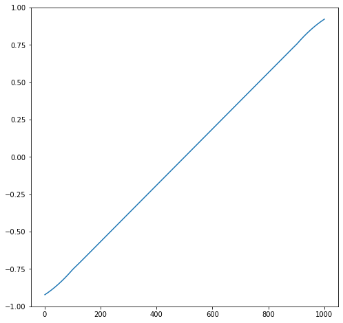
v = np.linalg.inv(A) @ b[:, None]
This looks like the plot in the book.
plt.figure(figsize=(8, 8))
plt.ylim([-1, 1])
plt.plot(state_idx, v);
Gradient Monte Carlo Algorithm for Estimating $\hat{v} = v_\pi(s)$
First for convenience we will create a new dict where the terminal states are also included among the neighbours representing $L$ by 0 and $R$ by 1. We also store the policy values correponds to each neighbour.
neighbours_with_terminal = dict()
policy = dict()

for i in neighbours:
    Ni = neighbours[i]
    pol = np.ones(len(Ni)) / 200.
    if (1000 - i) < 100:
        Ni = np.concatenate([Ni, [1001]])
        pol = np.concatenate([pol, [1 - np.sum(pol)] ])
    elif i <= 100:
        Ni = np.concatenate([[0], Ni])
        pol = np.concatenate([[1 - np.sum(pol)], pol])

    assert np.isclose(np.sum(pol), 1), (np.sum(pol), i, len(Ni))
    neighbours_with_terminal[i] = Ni
    policy[i] = pol
Now we can implement the following algorithm
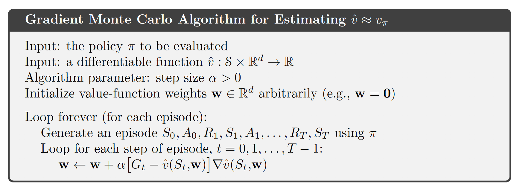
For this we use state aggregation where the states (excluding non-terminal whose values are known and will not be estimated) are divided into blocks of 100 consecutive states 1-100, 101-200, etc. and for each of these we have a single value parameter. The parameters here are simply the estimates of the value.
\(i_s = \left \lfloor{\frac{s}{100}}\right \rfloor\) \(\hat{v}\left(s, \mathbf{w}\right) = \mathbf{w}_{i_s}\)
Thus element $i_s$ of $\nabla\hat{v}\left(s, \mathbf{w}\right)$ is 1 and the rest are 0.
v_est = np.zeros(10)
alpha = 2e-5
episodes = 100_000
gamma = 1
num_visits = np.zeros(len(state_idx))

import sys


import tqdm
for episode in range(episodes):
    states = [500]
    actions = []
    rewards = []

    while True:
        s = states[-1]
        a = np.random.choice(
            neighbours_with_terminal[s],
            p = policy[s])
        actions.append(a)
        s_next = a
        states.append(s_next)
        r = 1*(s_next==1001) - 1*(s_next==0)
        rewards.append(r)

        if s_next in [0, 1001]:
            break

        num_visits[s_next - 1] += 1

    assert (len(states) - len(actions)) == 1
    assert (len(states) - len(rewards)) == 1

    # Remember rewards[0] represents R1 not R0
    returns = np.cumsum(rewards[::-1])[::-1]


    for st, gt in zip(states, returns):
        group_idx = (st - 1) // 100

        # Only update group_idx since grad is 0 for the others
        v_est[group_idx] += (alpha * (gt - v_est[group_idx]))


    if episode % 100 == 0:
        sys.stdout.write('\repisode {:06d} | '.format(episode) + (', '.join(['{:.4f}'] * 10)).format(*v_est))
episode 099900 | -0.8216, -0.6610, -0.4783, -0.2886, -0.0952, 0.0774, 0.2664, 0.4542, 0.6435, 0.82196000
The on-policy distribution in episodic tasks
The number of time steps spent on average in state $s$ is denoted as $\eta(s)$ and the probability that an episode starts at $s$ is denoted as $h(s)$
\[\eta(s) = h(s) + \sum_{\bar{s}}\eta\left(\bar{s}\right) \sum_a \pi\left(a \vert \bar{s}\right) p\left(s \vert \bar{s}, a\right), \forall s \in \mathcal{S}\]This defines a system of equations that can be solved for $\eta(s)$. Let us find this for the example above
B = np.zeros((1000, 1000))
h = np.zeros(1000)
h[500-1] = 1

for i in state_idx:
    Ni = neighbours[i]
    B[i-1, i-1] = 1
    # p(s|s',a) = 1 if a=s else 0
    # pi(s|s') = 1/200. if s' in Ni else 0
    B[i-1, Ni-1] = -1/200.
true_N = np.linalg.inv(B) @ h
The on-policy distribution $\mu(s)$ is just $\eta(s)$ normalised to sum to 1
\[\mu(s) = \frac{\eta(s)}{\sum_{s'}\eta(s')}\]true_mu = true_N / true_N.sum()
Putting everything together
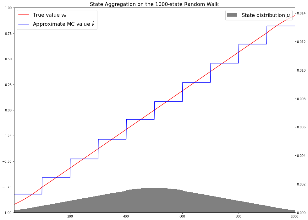
Now we have all the ingredients needed to make a plot like the one shown in Figure 9.1 in the book. Note the staircase shape of the estimate value function due to state aggregation. I highly recommend reading the full description of the example in the book to get a better understanding of what this figure shows.
plt.figure(figsize=(16, 12))


plt.ylim([-1, 1])
plt.plot(state_idx, v, color='red', label='True value $v_\pi$');
plt.plot(state_idx, np.repeat(v_est, 100), color='blue'
        , label='Approximate MC value $\hat{v}$');
plt.legend(fontsize=16);

plt.title('State Aggregation on the 1000-state Random Walk', fontsize=16)

ax = plt.gca().twinx()
ax.set_xlim([1, 1000]);
ax.bar(state_idx, true_mu, color='gray', label='State distribution $\mu$', width=1);
ax.legend(fontsize=16);
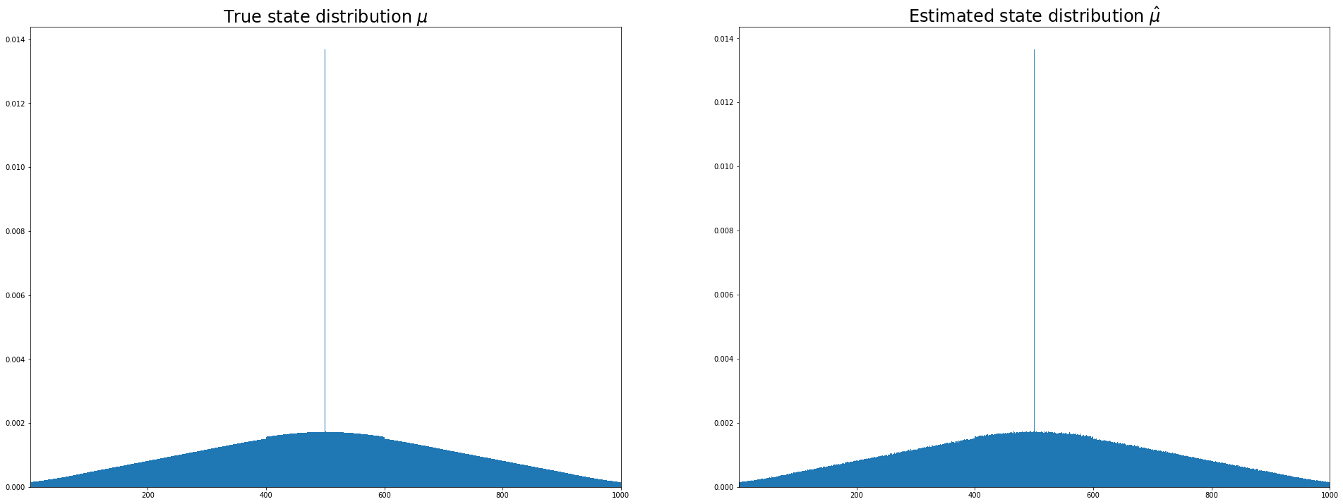
We can also compare the true on-policy distribution with the fraction of state visits and we find that they are very close.
# Always starts at 500 so add that
start_count = np.zeros(len(state_idx))
start_count[500-1] = episodes
num_visits_incl_start = start_count + num_visits
frac_visit = num_visits_incl_start / num_visits_incl_start.sum()
true_mu[500-1], frac_visit[500-1]
(0.013692348308814472, 0.01366513851646612)
fig, (ax1, ax2) = plt.subplots(1, 2, figsize=(33, 12))
ax1.bar(state_idx, true_mu, width=1);
ax2.bar(state_idx, frac_visit, width=1);
ax1.set_title('True state distribution $\mu$', fontsize=24);
ax2.set_title('Estimated state distribution $\hat{\mu}$', fontsize=24);
ax1.set_xlim([1, 1000])
ax2.set_xlim([1, 1000]);