A popular metric for evaluating image generation models is the Fréchet Inception Distance (FID). Like the Inception score, it is computed on the embeddings from an Inception model. But unlike the Inception score, it makes use of the true images as well as the generated ones. In the post we will learn how to implement it in PyTorch.
Contents
Let $p_w$ be the real world data distribution and $p$ the generated data distribution, with mean, covariance $\left(\mathbf{m}_w, \mathbf{C}_w\right)$ and $\left(\mathbf{m}, \mathbf{C}\right)$.
The Fréchet distance between a pair of Gaussians with parameters $\left(\mathbf{m}_w, \mathbf{C}_w\right)$ and $\left(\mathbf{m}, \mathbf{C}\right)$ is given by
\[d\left(\left(\mathbf{m}, \mathbf{C}\right), \left(\mathbf{m}_w, \mathbf{C}_w\right)\right) = \left\lVert \mathbf{m} - \mathbf{m}_w\right\rVert_2^2 + \text{Tr}\left(\mathbf{C} + \mathbf{C}_w - 2\left(\mathbf{C}\mathbf{C}_w\right)^\frac{1}{2}\right)\]To compute the Fréchet Inception distance Inception features are used to find the covariance and the mean.
Implementation
$\def\half{\frac{1}{2}}$ $\def\C{\mathbf{C}}$ $\def\Cw{\C_w}$ $\def\CCwh{\left(\C\C_w\right)^\half}$ $\newcommand\trace[1]{\text{Tr}\left({#1}\right)}$
First we need to get Inception features. In the paper that introduced FID, they write
For computing the FID, we propagated all images from the training dataset through the pretrained Inception-v3 model following the computation of the Inception Score … however, we use the last pooling layer as coding layer.
Here we will use the pretrained model from torchvision and replace the last fully connected layer with an Identity layer so that we get the pooled outputs from the last pooling layer.
def get_model():
    device = 'cuda' if torch.cuda.is_available() else 'cpu'
    model = torchvision.models.inception_v3(weights=torchvision.models.Inception_V3_Weights.IMAGENET1K_V1)
    # Hack to get features
    model.fc = torch.nn.Identity()
    return model
Now let us implement a function that calculates the covariance and the mean. Given features $X_i$ for example $i$
\[E\left[X\right] \approx \hat{E}\left[X\right] = \frac{1}{N}\sum_{i=1}^N X_i \\\\\\ \text{cov}\left(X\right) = E\left[XX^T\right] - E\left[X\right]E\left[X\right]^T \approx \frac{1}{N}\sum_{i=1}^N X_i X_i^T - \hat{E}\left[X\right] \hat{E}\left[X\right] ^T\]It will do this in a batched fashion, obtaining the features, then updating the sum of the features $X$ and the sum of $XX^T$ whilst keeping tracking of total number of inputs seen so far.
def get_moments(samples, model):
    device = 'cuda' if torch.cuda.is_available() else 'cpu'
    model.to(device)
    model.eval()

    with torch.no_grad():

        X_sum = torch.zeros((2048, 1)).to(device)
        XXT_sum = torch.zeros((2048, 2048)).to(device)
        count = 0

        for inp in tqdm.tqdm(samples):
          # [B, F]
          pred = model(inp.to(device))
          # [B, F] -> [1, F] -> [F, 1]
          X_sum += pred.sum(dim=0, keepdim=True).T
          # [B, 1, F] x [B, F, 1] -> [B, F, F] -> [F, F]
          XXT_sum += (pred[:, None] * pred[..., None]).sum(0)
          count += len(inp)

    # [F, 1]
    mean = X_sum / count
    # [F, F] - [F, F] -> [F, F]
    cov = XXT_sum / count - mean @ mean.T

    return mean, cov
Given the moments we can obtain the Fréchet Inception distance. Note that
\[\trace{\C + \Cw - 2\CCwh} = \trace{\C} + \trace{\Cw} - 2\trace{\CCwh}\]The first two terms are straightforward to evaluate. To obtain $\trace{\CCwh}$ note the sum of the eigenvalues of a matrix is equal to its trace. It can be shown that since both $\C$ and $\Cw$ are covariance matrices $\CCwh$ has ab eigenvalue matrix $D^\half$ where $D$ is the eigenvalue matrix of $\C\Cw$. Moreover, the eigenvalues of $\C\Cw$ are real and positive which means that the eigenvalues of $\CCwh$ are real. See the Appendix for more details.
def frechet_inception_distance(m_w, C_w, m, C, debug=False):
    eigenvals = torch.linalg.eigvals(C @ C_w)
    trace_sqrt_CCw = eigenvals.real.clamp(min=0).sqrt().sum()
    if debug:
        print('Largest imaginary part magnitude:', eigenvals[eigenvals.imag > 0].abs().max().item())
        print('Most negative:', eigenvals[eigenvals.real < 0].real.min().item())
    fid = ((m - m_w)**2).sum() + C.trace() + C_w.trace() - 2 * trace_sqrt_CCw
    return fid
Note that although theoretically real and non-negative the eigenvalues might have small complex parts due to floating point errors. Values close to 0 might also be represented as tiny negative numbers necessitating clamping to 0 and higher.
Example
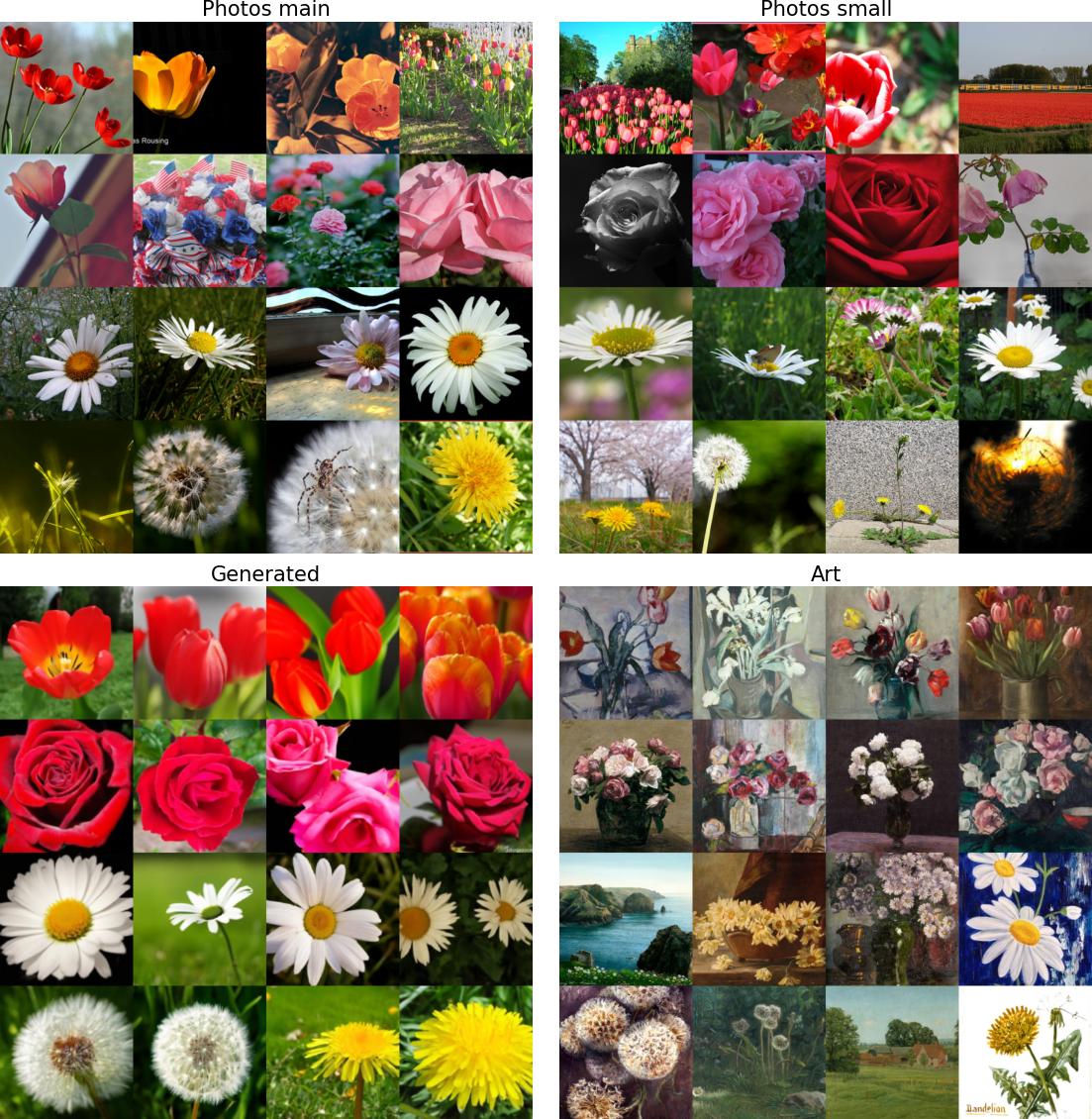
TF Flowers is dataset containing photographs for four types of flowers: roses, tulips, daisies and dandelions. We split this into two disjoint parts a large one used as the reference dataset of “true samples” and a small one. We compare three datasets to the reference dataset
- The smaller subset of TF Flowers
- Samples of all the flower types generated by a small GLIDE model
- Paintings of all four types of flowers
The FID of these datasets is as follows:
| Dataset | FID |
|---|---|
| Photos small | 71.61 |
| GLIDE samples | 116.71 |
| Art | 162.6 |
Since the datasets involved are one or two orders of magnitude smaller compared to the sizes typically used in literature, these results
Unsurprisingly the small photos dataset has the best FID (lower is better), followed by the photo-realistic GLIDE samples whilst the paintings have the highest FID. GLIDE images were generated with the prompt of the form “a photo of a rose” and “a photo of roses” with half of the images generated using each prompt type. As you can see most of the images show relatively close up images and only a small number of flowers. It is possible that more diverse prompts might result in an improved FID. It is interesting that the painting dataset often shows the flowers as part of a scene and in this respect is more similar to the photos dataset. However the appearance seems to be sufficiently different to lead to large FID.
Resources
Here are the links to resources used to generate these results. I have not shared the datasets except for the generated samples but you should be able to generate them yourself
- Colab used to generate the results above
- Folder with GLIDE generated images
- Download TF Flowers from here
- This Github gist contains the urls for the flower paintings which were downloaded from Art UK and the code used to download them(some of these are copyrighted so please check if they will be suitable for your purposes).
Appendix
We wish to show that if $A$ and $B$ are covariance matrices then
- $AB$ is diagonalisable
- $\left(AB\right)^\half$ has real eigenvalues
Preliminaries
- A covariance matrix $\Sigma$ has the form $E\left[(x - \bar{x})(x - \bar{x})^T\right]$ where $x$ is a random vector and $\bar{x} = E\left[x\right]$
- It is real since $x$ is real
- It is symmetric because \(\Sigma_{ij} = E\left[(x_i - \bar{x}_i)(x_j - \bar{x}_j)\right] = E\left[(x_j - \bar{x}_j)(x_i - \bar{x}_i)\right] = \Sigma_{ji}\)
- It is positive semi-definite (PSD) since
1. $AB$ is diagonalisable
- Since $A$ and $B$ are both symmetric and positive semi-definite, $AB$ is similar to a real symmetric PSD matrix, $B^\half A B^\half$ sharing the eigenvalues of this matrix (see also this)
- $B^\half A B^\half$ is symmetric since $A$ is symmetric and $B^\half$ is also symmetric (see this and this)
- $B^\half A B^\half$ is PSD because $B^\half$ is symmetric and $A$ is $PSD$ so that
\(\forall x. \text{ }\text{ } x^T{B^\half}A{B^\half}x = x^T\left({B^\half}\right)^T A{B^\half}x = \left({B^\half}x\right)^TA\left({B^\half}x\right) \geq 0\)
- Since $AB$ is similar to a real symmetric matrix it is diagonalisable
2. $\left(AB\right)^\half$ has real eigenvalues
- A matrix is $X$ is said to be diagonalisable if it can be written in the form $VDV^{-1}$, where $D$ is the diagonal eigenvalue matrix of $X$ and the columns of $V$ are the eigenvectors of $X$
-
A square root of a diagonalisable matrix can be written in the form $VD^\half V^{-1}$ where $D^\half$ is a diagonal matrix such that $D^\half_{ii} = \sqrt{D_{ii}}$ which are the eigenvalues of $\left(AB\right)^\half$
- $AB$ shares the eigenvalues of $B^\half A B^\half$ which is a PSD matrix and therefore has real and non-negative eigenvalues
- This means that the eigenvalues of $\left(AB\right)^\half$ are real