$\def\ttheta{\boldsymbol{\theta}}$
import numpy as np
import matplotlib.pyplot as plt
In the previous post we introducted the short-corridor gridworld with switched actions from Example 13.1 Reinforcement Learning (Sutton and Barto)

- The start state is S
- The terminal state is G
- There are two possible actions $L$ (move left) and $R$ (move right)
- The reward for each transition is -1 until G is reached
- In all but the second state chosen the action $L$ moves to the state on the left if one eixsts otherwise remains in the same state, and similarly for $R$
- In the second state the actions have flipped outcomes: $R$ moves to the state on the left and $L$ to the state on the right
Previously we found an analytical solution for the probability for moving right. Now we will use the REINFORCE algorithm to solve this problem.
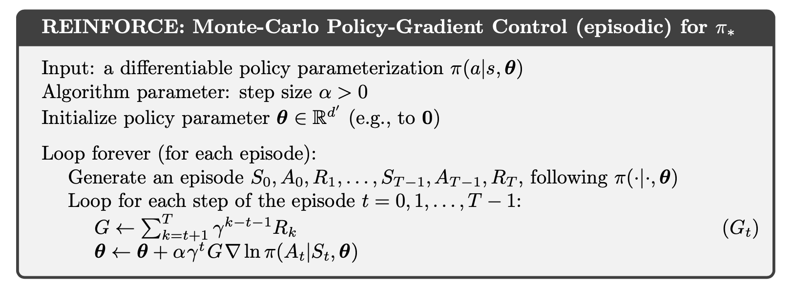
This is a situation where with a discrete as well as small action space (move left or right). Consequently a suitable policy parameterization is a softmax over action preferences
\[\pi\left(a \vert s, \ttheta\right) = \frac{e^{h\left(s, a, \ttheta\right)}}{\sum_b e^{h\left(s, b, \ttheta\right)}} \\\\\\ h\left(s, a, \ttheta\right) = \theta^T\mathbf{x}\left(s,a\right)\]where $\mathbf{x}\left(s,a\right)$ is a feature vector.
def policy(t, feature):
    logits = t @ feature
    logits_exp = np.exp(logits - np.max(logits, -1, keepdims=True))
    # [T, [pR, pL]]
    pi = logits_exp / logits_exp.sum(-1, keepdims=True)
    return pi
We are going to implement a vectorised version of REINFORCE to enabling running several trials at once whose results will then be averaged. The states will be numbered 1 to 4 from left to right
                    1       2       3       4
                +-------+-------+-------+-------+
                |   S   | <---. |       |       |
                | <-o-> | .-o-' | <-o-> |   G   |
                |       | '---> |       |       |
                +-------+-------+-------+-------+
The feature vectors $\mathbf{x}\left(s,a\right)$ are one hot vectors and they don’t depend on the state
\[x(s, R) = [0, 1]^T \\\\\\ x(s, L) = [1, 0]^T\]x_sR = np.array([[1], [0]])
x_sL = np.array([[0], [1]])
# [2, 2]
X = np.concatenate([x_sR, x_sL], axis=-1)
For $\alpha$ we will try three values: $2^{-12}, 2^{-13}, 2^{-14}$
alpha_powers = [-12, -13, -14]
num_alpha = len(alpha_powers)
episodes = 1000
trials = 100
max_steps = 1000
result = np.zeros([num_alpha, trials, episodes, 2])
G0 = np.zeros([num_alpha, trials, episodes])
To handle having different random seeds for each trial, we can create a matrix of random values in advance from each seed and then used these to sample from the policy such that if the value is less that $\pi(R \vert s)$, $R$ is be chosen otherwise $L$ is chosen.
seeds = [np.random.randint(low=0, high=2**32) for run in range(trials)]
random_vals = np.zeros([num_alpha, trials, episodes, max_steps])
for t, s in enumerate(seeds):
    random_vals[:, t] = np.random.RandomState(s).uniform(size=random_vals[:, t].shape)
Now create a function that generates an episode for all the trials at once
def generate_episode(theta, X, random_values):
    """
    theta: [trials, num_actions]
    X: [num_actions, num_actions]
    random_values: [trials, max_steps]
    """

    trials, max_steps = random_values.shape

    # initialise arrays
    states = [np.ones(trials)]
    actions = []
    rewards = []

    # keep track of whether the terminal state has been reached for each trial
    inprog = [np.ones(trials).astype('bool')]

    step = 0

    while inprog[-1].any() and step < max_steps:
        s = states[-1]

        # Find probability of going right according to policy
        pi = policy(theta, X)
        pR = pi[:, 0]

        # 1 for right, -1 for left
        a = np.where(random_values[..., step] < pR, 1, -1)
        actions.append(a)

        # To flip action for state 2
        coef = np.where(s==2, -1, 1)

        # If in progress, update by moving left or right,
        #  flipping for state 2 and disallowing moving
        #  left from state 1
        # If not in progress, remain in state 4 which is
        #   the terminal state
        s_next = np.where(inprog[-1], np.maximum(coef * a + s, 1), 4)
        states.append(s_next)

        # Reward is -1 until terminal state when it is 0
        rewards.append(-np.ones(trials) * inprog[-1].astype('float'))
        inprog.append((s_next!=4))

        step += 1

    return states, actions, rewards, inprog
Then we can implement the second part. Following the “official” (and non-vectorised) implementation on the RL book website we have $\gamma = 1$.
def update_parameters(theta, X, alpha, states, actions, returns, inprog):

    # Calculate returns in advance
    returns = np.cumsum(rewards[::-1], axis=0)[::-1]

    for prog_t, st, gt, at in zip(inprog, states, returns, actions):
        # R=1 -> 0, L=-1 -> 1
        act_idx = (at < 0).astype('int')

        # [T, 2]
        x_sa = X.T[act_idx]

        # [T, 2]
        pi = policy(theta, X)

        # See Exercise 13.3
        # [T, 2] - [T, 2] -> [T, 2]
        ln_pi_grad = x_sa - pi @ X.T
        update = alpha * gt[:, None] * ln_pi_grad
        theta[prog_t] += update[prog_t]

    return theta.squeeze(), returns[0]
Now we can put these together to run the example. We initialise $\ttheta = [\ln(1), \ln(19)]$ also following the official implementation.
for idx, power in enumerate(alpha_powers):
    theta = np.tile(np.log([1, 19])[None], [trials, 1])
    alpha = 2**power

    for episode in range(episodes):
        states, actions, rewards, inprog = generate_episode(theta, X, random_vals[idx, :, episode])
        result[idx, :, episode], G0[idx, :, episode] = update_parameters(theta, X, alpha, states, actions, rewards, inprog)

        if episode % 100 == 0:
            print(f'alpha=2^{power}, episode={episode + 1}', policy(theta, X).mean(0).squeeze())
alpha=2^-12, episode=1 [0.05137732 0.94862268]
alpha=2^-12, episode=101 [0.2730593 0.7269407]
alpha=2^-12, episode=201 [0.37056455 0.62943545]
alpha=2^-12, episode=301 [0.43080733 0.56919267]
alpha=2^-12, episode=401 [0.47190531 0.52809469]
alpha=2^-12, episode=501 [0.49833314 0.50166686]
alpha=2^-12, episode=601 [0.51648553 0.48351447]
alpha=2^-12, episode=701 [0.54041319 0.45958681]
alpha=2^-12, episode=801 [0.5450163 0.4549837]
alpha=2^-12, episode=901 [0.55932724 0.44067276]
alpha=2^-13, episode=1 [0.05070895 0.94929105]
alpha=2^-13, episode=101 [0.15114146 0.84885854]
alpha=2^-13, episode=201 [0.22269873 0.77730127]
alpha=2^-13, episode=301 [0.2788509 0.7211491]
alpha=2^-13, episode=401 [0.32195895 0.67804105]
alpha=2^-13, episode=501 [0.35928062 0.64071938]
alpha=2^-13, episode=601 [0.39119684 0.60880316]
alpha=2^-13, episode=701 [0.41764465 0.58235535]
alpha=2^-13, episode=801 [0.44153935 0.55846065]
alpha=2^-13, episode=901 [0.45895968 0.54104032]
alpha=2^-14, episode=1 [0.05057726 0.94942274]
alpha=2^-14, episode=101 [0.09540479 0.90459521]
alpha=2^-14, episode=201 [0.13557795 0.86442205]
alpha=2^-14, episode=301 [0.17262241 0.82737759]
alpha=2^-14, episode=401 [0.20356134 0.79643866]
alpha=2^-14, episode=501 [0.23276498 0.76723502]
alpha=2^-14, episode=601 [0.25941758 0.74058242]
alpha=2^-14, episode=701 [0.28391618 0.71608382]
alpha=2^-14, episode=801 [0.30547963 0.69452037]
alpha=2^-14, episode=901 [0.32668467 0.67331533]
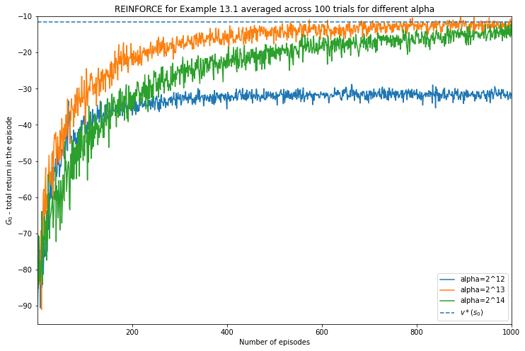
Finally we plot the averaged values which can be compared to value using the optimal choice for the probability to move the right that we derived earlier.
v_best = -11.65685424949238 # from before
plt.figure(figsize=(12,8))
for i in range(3):
    plt.plot(np.arange(episodes) + 1, G0[i].mean(0), label=f'alpha=2^{12 + i}')

plt.title('REINFORCE for Example 13.1 averaged across 100 trials for different alpha')
plt.ylabel('$G_0$ - total return in the episode')
plt.xlabel('Number of episodes')
plt.xlim([1, episodes])
plt.ylim([-95, -10])
plt.hlines(xmin=1, xmax=episodes, y=v_best, label='$v*(s_0)$', linestyle='--');
plt.legend();