In an earlier post about we learned about diffusion models, a new and powerful type of generative model that most notably is the basis for OpenAI’s DALL-E 2. However an important disadvantage with these models is that a large number forward passes - typically 1000 or more - are needed to generate samples, making inference slow and expensive. In this post we will look at a couple of different methods that have been developed to speed up inference.
Methods like DDIM allow you to generate 20 or more images of comparable quality in the time it would take to generate a single one using the original sampling technique
- The first approach DDIM is theoretically motivated and is based on the argument that the weights of the trained model are optimal for a whole family of reverse processes, some of which may involve an order of magnitude fewer sampling steps.
- The other approach is empirical and is not unlike downsampling, where you can take fewer samples but still get good results
Contents
Denoising diffusion implicit models
The reason inference is slow is because the sampling process reverses the forward process which has $T$ timesteps. A key insight from the paper “Denosing Diffusion Implicit Models” (DDIM) is that the objective $L_\text{simple}$ only depends on $\qrcond{\xt}{\xz}$ and not on the joint distribution $\qrcond{\xoneT}{\xz}$. This means that there could be other inference processes - including those that need fewer steps - which could have the same marginals.
Non-Markovian forward process
One approach is to define a family of distributions indexed by $\sigma$
\[q_\sigma\left(\xoneT\vert\xz\right) = q_\sigma\left(\xtt{T} \vert\xz\right) \prod_{t=2}^Tq_\sigma\left(\xtmone \vert\xt, \xz\right)\]where $q_\sigma\left(\xtmone \vert\xt, \xz\right)$ is Gaussian
\[\qrsigcond{\xoneT}{\xz} = \qrsigcond{\xtt{T}}{\xz}\prod_{t=2}^T\qrsigcond{\xtmone}{\xt, \xz}\]From this a new non-Markovian forward process is derived using Bayes rule
\[\qrsigcond{\xtt{1}}{\xtmone, \xz} = \frac{ \qrsigcond{\xtmone}{\xt, \xz}\qrsigcond{\xt}{\xz}}{ \qrsigcond{\xtmone}{\xz} }\]It is not Markovian since $\xt$ depends on $\xz$ as well as $\xtmone$. However the parameters of $q_\sigma\left(\xtmone \vert\xt, \xz\right)$ are chosen such that $q_\sigma\left(\xt \vert \xz\right)$ is the same as in the original Markovian forward process.
Now we can define a new reverse distribution based on $q_\sigma\left(\xtmone \vert \xt, \xz\left(\xt\right)\right)$. As before we can estimate $\xz$ given $\xt$. Define $f_\theta^{(t)}\left(\xt\right) := \frac{1}{\abt}\left(\xt - \sqrt{1 - \abt}\etta\left(\xt, t\right)\right)$. Then the reverse process is defined as
\[p_\theta^{(t)}\left(\xtmone \vert \xt\right) = \left\{ \begin{array}{ll} \norm{f_\theta^{(1)}\left(\xtt{1}\right), \sigma_1^2\II} & \text{if }{t=1} \\ q_\sigma\left(\xtmone \vert \xt, f_\theta^{(t)}\left(\xt\right)\right) & \text{otherwise} \end{array} \right.\]Sampling
To sample from the reverse process you started off with a noise sample $\xtt{T} \sim \norm{\mathbf{0}, \II}$, successively sampling
\[\xtmone = \sqrt{\frac{\abtmone}{\abt}}\left(\xt - \sqrt{1 - \abtmone}\etta\left(\xt, t\right)\right) + \sqrt{1 - \abtmone - \sigma_t^2}\etta\left(\xt, t\right) + \sigma_t\epsilon_t\]The hyperparameter $\sigma_t$ controls the stochasticity of the process:
- $\sigma_t = \sqrt{ (1 - \abtmone)(1 - \abt)\left(1 - \frac{\abt}{\abtmone}\right) }$ for all $t$ yields the DDPM model.
- $\sigma_t = 0$ for all $t$ leads to a result that is deterministic given $\xtt{T}$ and the resulting model is called the denoising diffusion implicit model.
Accelerated inference
In fact we can use any forward process provided that the marginals match. This allows the use of a forward process defined only on a subset of the latent variables
\[\xtt{\tau_1} \ldots \xtt{\tau_t}\]where $\tau_1 \ldots \tau_t$ is an increasing sub sequence of $1 \ldots T$ with of length $S$ where $S$ could be much smaller that $T$. The corresponding reverse process goes backwards through the timesteps
\[\xtt{ \tau_{t - 1}} = \sqrt{\frac{\abtautmone}{\abtaut}}\left(\xtt{\tau_t} - \sqrt{1 - \abtaut}\etta\left(\xtt{\tau_t}, \tau_t\right)\right) + \sqrt{1 - \abtautmone - \sigma_{\tau_t}^2}\etta\left(\xtt{\tau_t}, \tau_t\right) + \sigma_{\tau_t}\epsilon_t \\\\\\ t = 1 \ldots S\]Using existing diffusion models
Another key advantage of this approach is that you can simply use an existing diffusion model trained on the DDPM objective and don’t need to do further training. In the DDIM paper the reasoning for this is as follows
- The simplified loss as we saw in the previous post has the form $$L_\text{simple}\left(\theta\right) := \Ef{t, \xz, \boldeps}{\left\Vert\boldeps - \etta\left(\sqrt{\abt}\xz + \sqrt{1-\abt}\boldeps\right)\right\Vert^2} \\ \propto \sum_{t=1}^T\Ef{\xz, \boldeps}{\left\Vert\boldeps - \etta\left(\sqrt{\abt}\xz + \sqrt{1-\abt}\boldeps\right)\right\Vert^2} $$
- since $t$ is sampled uniformly
- This came about after we approximated $L_0$ and dropped the timestep-dependent weights for $L_t$ for all $t$ which have the form $\frac{\bt^2}{2\sigma^2\at(1 - \abt)}$
- Supposing the parameters of the noise model $\etta$ were not shared across timesteps, then each term in sum could be optimised independently and the optimal value of the parameters $\theta$ would not be influenced by the weights.
- This is true for any set of timestep-dependent weights, $\gamma$
- Denote by $L_\gamma$ the loss associated with these weights and note that $L_\text{simple} = L_1$
- It can be shown that the variational lower bound for new model $$J_\sigma = \Ef{\xtt{0:T}\sim q_\sigma\left(\xtt{0:T}\right)}{\log q_\sigma\left(\xoneT\vert\xz\right) - \log p_\theta\left(\xtt{0:T}\right)} = \text{const}. + L_\gamma$$
- for some $\gamma$ (this is Theorem 1 in the DDIM paper - see Appendix B in the paper for a derivation)
- This means that minimising $L_1$ and therefore $L_\gamma$ also minimises $J_\sigma$
However in the DDPM paper the parameters are shared across timesteps which means that $\sum_{t=1}^T\Ef{\xz, \boldeps}{L_t}$ is only an approximation to the loss. Consequently the reasoning above does not strictly hold with regard to the actual implementation. Nevertheless, as with so many things in deep learning, using a pre-trained model works in practice.
Implementation
In the paper they experiment with a linear and quadratic sequence for the timesteps. Here we will focus on the linear sequence. In the paper this is defined as $\lfloor ci \rfloor$. We will use the approach in the improved_diffusion codebase
def space_timesteps(
    num_sample_steps = 50,
    total_steps = 1000
):
    """
    Adapted from `improved_diffusion.respace.space_timesteps`
    """
    for i in range(1, total_steps):
        if len(range(0, total_steps, i)) == num_sample_steps:
            return list(range(0, total_steps, i))[::-1]

    raise ValueError(f'cannot create exactly {total_steps} steps with an integer stride')
To sample you would loop through pairs $(\tau_t, \tau_{t-1})$
timesteps = get_timesteps(S, T)
tau = timesteps[:-1]
tau_prev = tau[1:]
for t, tau_t, tau_tm1 in zip(range(len(tau), 0, -1), tau, tau_prev):
    ## CODE FOR SAMPLING GOES HERE
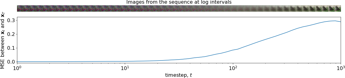
When the model has been trained, we can sample new data points by first sampling random noise $\xtt{\tau_t}$, then successively sampling latents at points $\tau_t$ along the sequence, $\xtt{\tau_t}$. As you can see in the figure below, if $\tau_t < T$ provided it is large enough $\xtt{\tau_t}$ will be very noisy and reasonably similar to $\xtt{T} \sim \norm{\mathbf{0}, \II}$ so random noise can be used as the initial value.
Assume we have $\xtt{\tau_t}$. To start with we sample $\xtt{\tau_t} \sim \norm{\mathbf{0}, \II}$
def p_sample_step(self, t, tau_t, tau_tm1, xtau_t):
Predict $\etta\left(\xtt{\tau_t}, \tau_t\right)$
    batch_shape = tf.shape(xtau_t)

    eps_theta = self.model(
        self.get_input(xtau_t, tau_t), training=False
    )
Transform this to $\xz = \frac{1}{\abtaut}\left(\xtt{\tau_t} - \sqrt{1 -\abtaut}\etta\left(\xtt{\tau_t}, \tau_t\right)\right)$. Clip to the range $[-1, 1]$ to get the prediction for $\xz$ that will be returned.
    predicted_x0 = (
        xtau_t - self.select_timestep(self.sqrt_1_m_alpha_bar, tau_t, xtau_t) * eps_theta
    ) / self.select_timestep(self.sqrt_alpha_bar, tau_t, xtau_t)
    x0 = tf.clip_by_value(predicted_x0, -1, 1)
$\def\dirxt{\sqrt{1 - \abtmone - \sigma_{\tau_t}^2}\cdot\etta\left(\xtt{\tau_t}, \tau_t\right)}$
Calculate direction pointing to $\xt$
\[\dirxt\]
    sigma_tau_t = self.select_timestep(self.sigma, tau_t, xtau_t)

    xtau_t_dir = tf.math.sqrt(
        1 - self.select_timestep(
            self.alpha_bar_prev, tau_tm1 + 1, xtau_t
        ) - sigma_tau_t ** 2
    ) * eps_theta
$\def\predxz{\underbrace{\frac{\xt - \sqrt{1 - \abt}\etta\left(\xtt{\tau_t}, \tau_t\right)}{\abtaut}}_\text{predicted $\xz$}}$
For $t > 1$, sample $\boldeps \sim \norm{\mathbf{0},\II}$ and return
\[\xtt{\tau_{t-1}} = \frac{1}{\abtautmone}\predxz + \underbrace{\dirxt}_\text{direction pointing to $\xtt{\tau_t}$} +\sigma_{\tau_t}\epsilon_t\]which is a sample from $\qrcond{\xtt{\tau_{t-1}}}{\xz}$. At the final step, $t=1$, just return $\xz$.
    z = tf.cond(
        tf.greater(t, 1),
        lambda: tf.random.normal(shape=batch_shape),
        lambda: tf.zeros(batch_shape)
    )

    xtau_tm1 = self.select_timestep(
        self.sqrt_alpha_bar_prev, tau_tm1 + 1, xtau_t
    ) * predicted_x0 + xtau_t_dir + sigma_tau_t * z

    return x0, xtau_tm1
Performance
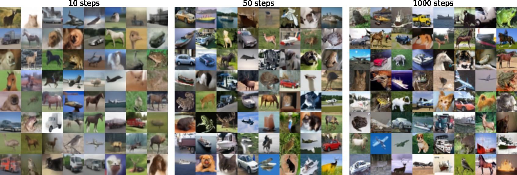
First let us look at some DDIM samples for CIFAR-10. The figure below shows samples with different initial values and visually there isn’t much of a difference in quality between 50 and 1000 and even using only 10 steps still yields tolerable images.
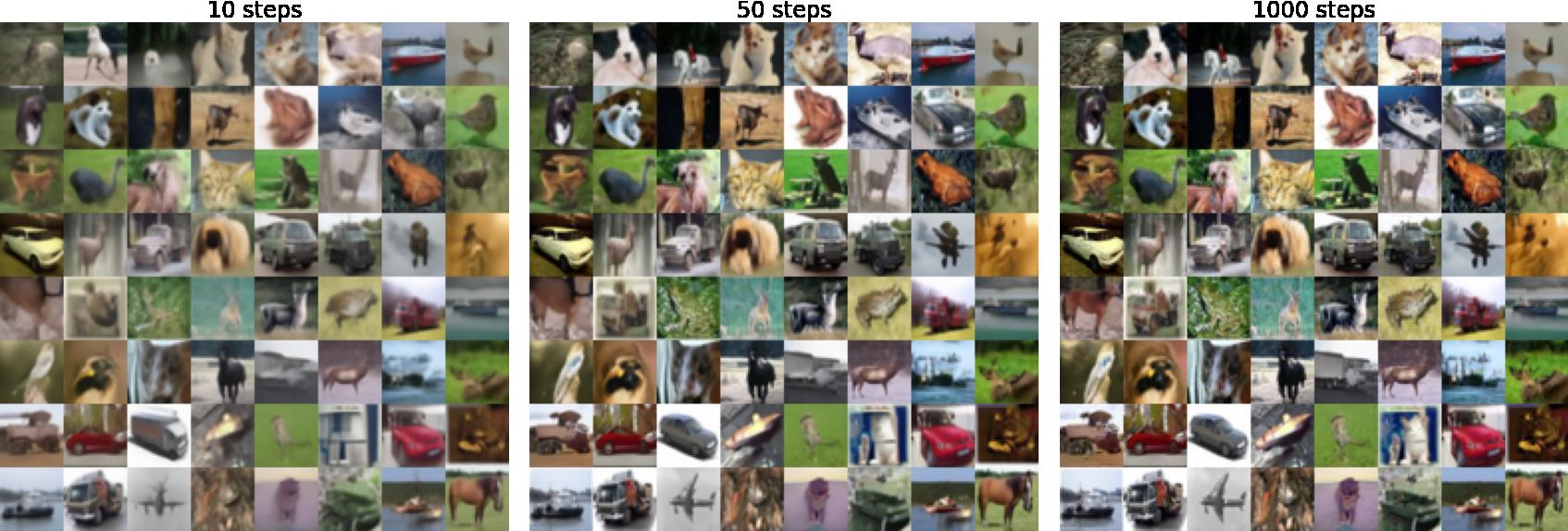
The images below were generated using the same initial random values. Here we see that just 50 steps is enough to get results that look not too different from 1000 steps. Using just 10 steps leads to much more blurry results.
This trend is more evident when we look at a single image
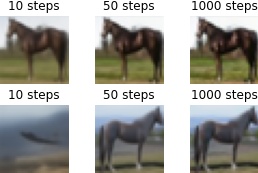
where the first example is blurry after ten steps whilst the second looks like an unfinished painting with most of the horse’s body absent except for some shadows and a slighlty pale region where its front hooves should be.
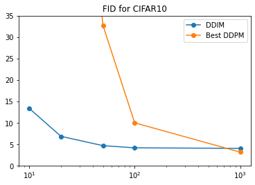
What about quantitative performance? I enourage you to refer to the paper for detailed information, figures and tables. But in summary, DDIM typically outperforms DDPM when only a small number of timesteps are used, 100 or less. However with 1000 timesteps, the same as training, DDPM does the best. Datasets consider include CIFAR-10, CelebA, LSUN. For example for CIFAR10, Frechet Inception Distance (FID) for DDIM and DDPM is 4.16 and 9.99 respectively with 100 sampling steps. However at a 1000 steps the score for DDIM only rises a little to 4.04 whilst for DDPM it plummets to 3.17.
Strided sampling
In the paper “Improved Denoising Diffusion Probabilistic Models” (Improved Diffusion) they show that you can actually get good results simply by sampling at points along a strided sequence $\tau$ from $1 \ldots T$ inclusive using hyperparameters indexed by $\tau_t$ and $\tau_{t-1}$ instead of $t$ and $t-1$ at step $t$. In the improved diffusion paper they introduce the following extensions to the original model (among others)
- A new noise schedule defined in terms of $\abt$ from which $\beta_t$ is derived according to the the definition $\beta_t = 1 - \frac{\abt}{\abtmone}$
- Learned variance parameterised as a learned interpolation between $\beta_t$ and $\tbt$
Accordingly when sampling at strided timesteps and using learned variance, $\beta_{\tau_t}$ and $\tilde{\beta}_{\tau_t}$ are derived as
\begin{align} \btaut = 1 - \frac{\abtaut}{\abtautmone}, && \tbtaut = \frac{1 - \abtaut}{1 - \abtautmone}\btaut \end{align}
They use a simple strided timestep sequence as follows
To reduce the number of sampling steps from $T$ to $K$, we use $K$ evenly spaced real numbers between 1 and $T$ (inclusive), and then round each resulting number to the nearest integer
which can be implemented as follows
timesteps = np.linspace(1, T, K).round().astype('int')
timesteps = np.unique(timesteps)[::-1]
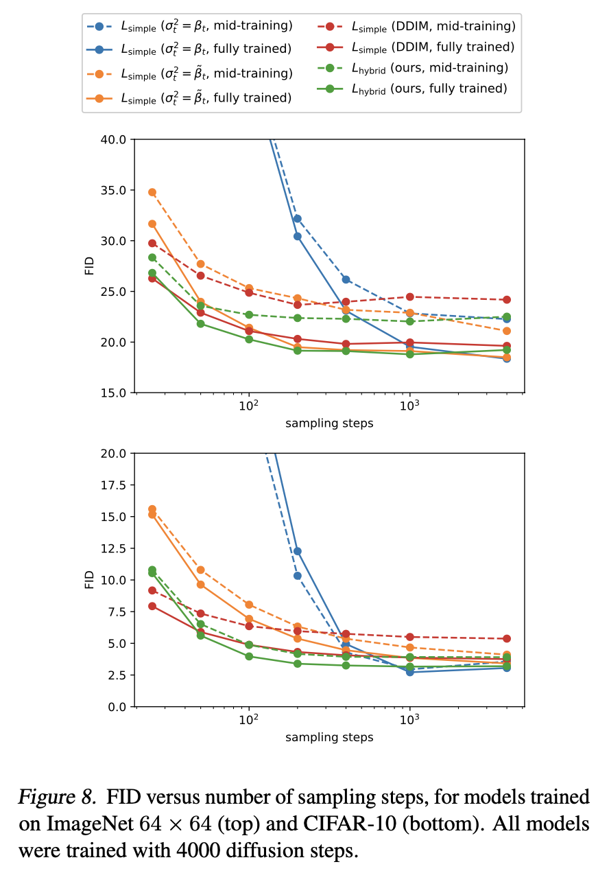
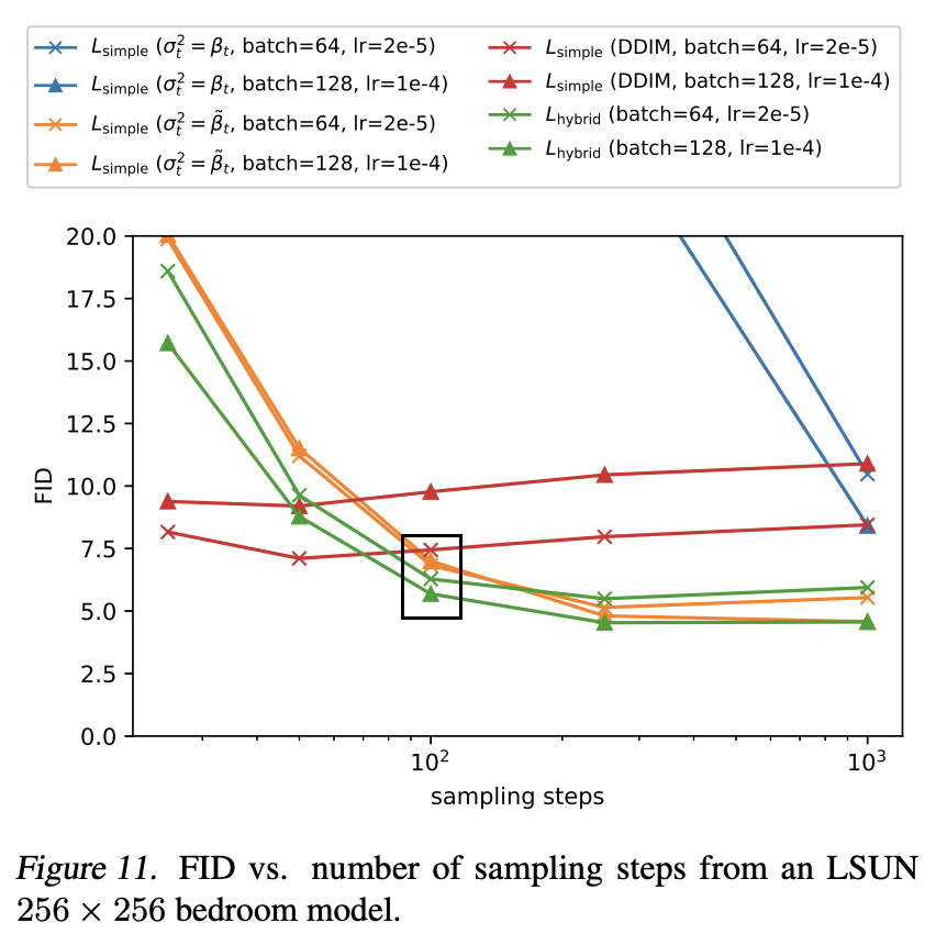
On the models developed in the Improved Diffusion paper, this method actually outperforms DDIM except when using fewer than 50 steps. At around 100 steps strided sampling leads to FID close to the optimal value. The paper claims that models with fixed variance
suffer much more in sample quality when using a reduced number of sampling steps
for both $\tbt$ and $\bt$. However the plots in the paper show that except for CIFAR-10, the difference in FID after around 100 steps is not large, when the fixed variance is $\tbt$ rather than $\bt$.