Non-maximum suppression (NMS)

6 min read July 20, 2021

Categories

• cv
• detection

This blogpost contains a quick practical introduction to a popular post-processing clustering algorithm used in object detection models. The code used to generate the figures and the demo can be found in this Colab notebook.

A problem of too many boxes

Suppose we are building an orange detector which identifies all the oranges growing in a tree. Maybe it is will be used by a fruit picking robot. One way to “find” orange is drawing boxes around orange-like regions of the image¹ and predicting the probability that the box contains an orange.

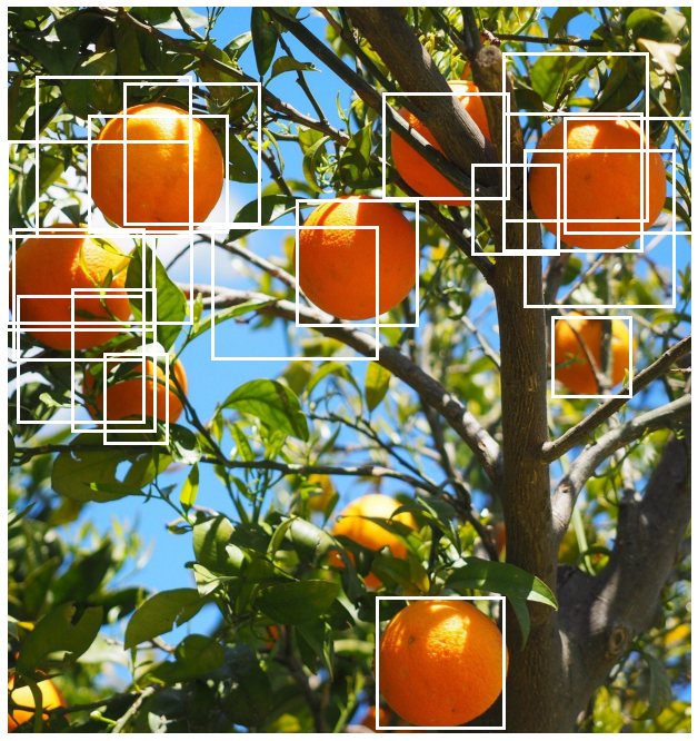
A common scenario in object detection models is that you end up with many overlapping detections as shown in the image below.

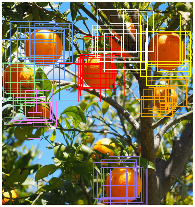
A good bounding box for a given object should contain as much of the object and as little of anything else as possible besides having a high probability predicted for the class of the object. The four sides of an ideal bounding box would be tangential to the uppermost, leftmost, lowermost and rightmost points of the object and have an associated probability prediction of 1 for the class of the object it contains.

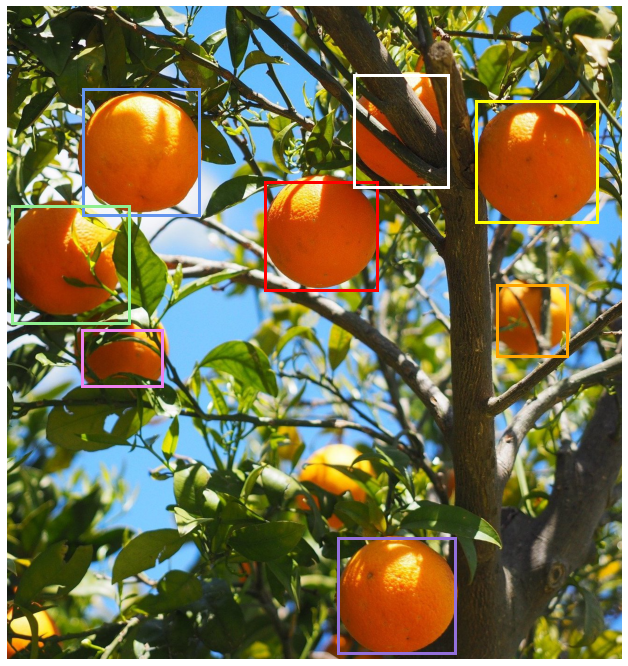
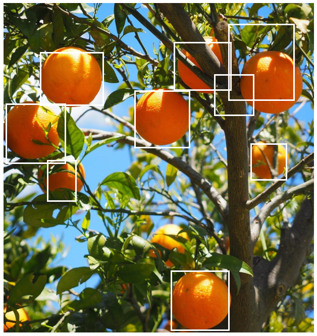
Some of detections above are evidently better than others. For example if you observe the lowermost orange fruit (with the violet bounding boxes) you can see that some of the boxes only cover about half of the orange. We would like to find a way to keep just the best ones, ideally just one detection per object. We want something that looks more like this:

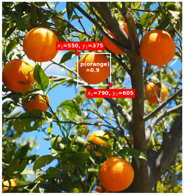
Typically each detection consists of

• A bounding box, represented for example by its top left and bottom right corners
• A set of score predictions for the possible classes of objects in the dataset - here we would just have two classes orange and not orange and one way the model could predict the score is to output a single score that is interpreted as the probablity that the object is orange.

(Sometimes it will have other attributes like additional properties and predictions, such as masks in an instance segmentation model, but we will focus on just scores and boxes here).

Simple methods like choosing just the top $N$ detections where $N$ is smaller than the total number of detections don’t make use of the location information. For instance all the top scoring detections could be in one region in the image even though there are predictions in other areas.

Looking at the image we see how the boxes are roughly clustered around the areas where oranges are present. Using location information we can group the bounding boxes so the ones that are sufficiently close to each another (according to some metric) will belong to a cluster. We can then aggregate the predictions within a cluster to get a single prediction per cluster.

Filtering detections with non-maximum suppression

A common algorithm is non-maximum suppression or NMS. There is more than one way to do this but here we will discuss the most frequently used approach which is a greedy algorithm.

It can be described very simply as follows:

• Sort the bounding boxes in descending order by their corresponding scores - sorted_boxes

• Initialise a top_boxes array

• Repeat the following until sorted_boxes is empty:

  • Pick the first bounding box, top_box, in the list and add to top_boxes.
  • Find the intersection over union (IoU) of top_box with each of sorted_boxes[1:]. IoU is the metric used to determine if boxes are “close” to each other. You can learn about how to calculate it efficiently here.
  • Identify all the boxes in sorted_boxes[1:] whose IoU with top_box is greater than or equal to threshold - these are the boxes in the same cluster as top_box.
  • Delete these cluster boxes along with top_box from sorted_boxes.

The boxes in top_boxes when the algorithm terminates represent the final predictions.

In practice you might also select other attributes such as score, segmentation, etc. associated with the bounding box and return them along with the boxes.

For this code² we use a box_iou function that is explained in detail in this post. Here all you should know is that, given a pair of array boxes1 of shape $N_1 \times 4$ and boxes2 of shape $N_2 \times 4$, will return an $N_1 \times N_2$ array ious where ious[i, j] is the intersection-over-union of boxes1[i] and boxes2[j]:

def nms(pred_boxes, pred_scores, threshold):
    assert 0 <= threshold <1
    sort_idx = np.argsort(pred_scores)[::-1]

    sorted_boxes = pred_boxes[sort_idx]
    sorted_scores = pred_scores[sort_idx]

    boxes_to_keep = []
    scores_to_keep = []

    while len(sorted_boxes) > 0:
        # Note that we include the top box in the IoUs to
        # simplify deleting it later.
        ious = box_iou(sorted_boxes[0], sorted_boxes).squeeze()

        boxes_to_keep.append(sorted_boxes[0])
        scores_to_keep.append(sorted_scores[0])

        # Since the top box has an IoU of 1 with itself,
        # it will also not be included here
        idx = np.where(ious < threshold)

        sorted_boxes = sorted_boxes[idx]
        sorted_scores = sorted_scores[idx]


    return np.array(boxes_to_keep), np.array(scores_to_keep)

NMS demo

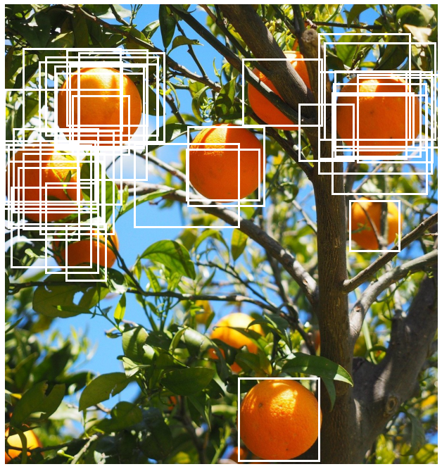
Let us now apply this function to our example using an IoU threshold of 0.9. This threshold basically says two boxes can be considered to belong to the same cluster only if the overlap of the boxes is at least 90% the total area covered by the boxes implying a high degree of overlap.

What we end up with looks better. In particular the fairly isolated orange towards the botttom of the image has just a single box around it but there are still a lot of boxes towards the top of image where there are quite a few oranges close to each other.

Notice also in the figure above that clusters formed the boxes prior to applying NMS are quite spread out which suggests that we should try relaxing the threshold for including a box in a cluster. The threshold is a hyperparameter whose optimal value depends on the dataset and needs to be tuned accordingly. Here let us try decreasing it to 0.5.

This has reduced the number of boxes but overlapping boxes still remain at the top right and left of the image. We will try decreasing the threshold again to 0.1.

This looks a lot better. Almost all the oranges have a box that bounds them reasonably well. However an extra box that overlaps with two of the other bounding boxes remains on the top-left. We also note how the orange at the top right of the image does not have such a tight bounding box.

As NMS is a greedy algorithm it sometimes fails to generate the best clusters. In the original set of boxes there were better bounding boxes for the top right orange but they were absorbed into one of the other clusters. This can happen when one detection has a box with that bounds the object best but another detection has a better score since higher scoring detections are prioritised by NMS.

Exercises

• As we noted, NMS is a clustering algorithm but in the version above we only make use of the prediction information associated with a single box in the cluster. Can you modify it so that it returns the averages of the scores and the bounding box coordinates per cluster?

• In practice you will often want to return indices so you that could select additional predictions associated with a detection that are not needed for NMS, such as masks, without needing to pass them into the NMS function. Can you modify the function so that it returns the sorted indices that index into the original input arrays?

• Take a look at the NMS implementation in a deep learning framework (for instance torchvision.ops.nms in Pytorch or tf.image.non_max_suppresion in TensorFlow). What arguments does it have and how do they differ from our simple implementation above?

Notes

1. Cropped from original image from Pixabay by Hans.
2. Code to generate the figures and run the demo can be found here.

Share Tweet LinkedIn Reddit