Contents
Introduction
In this blogpost we will implement Example 4.2: Jack’s Car Rental from Chapter 4 Reinforcement Learning (Sutton and Barto aka the RL book). This is an example of a problem involving a finite Markov Decision Process for which policy iteration is used to find an optimal policy.
I strongly suggest that you study Chapter 4 of the book and that you have a go at implementing the example yourself using this blogpost as a reference in case you get stuck.
Problem Statement
Here is a slightly modified version of the description of the problem given in Chapter 4.3 Policy Iteration of the RL book.
Example 4.2: Jack’s Car Rental
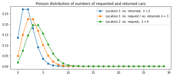
Jack manages two locations for a nationwide car rental company. Each day, some number of customers arrive at each location to rent cars. If Jack has a car available, he rents it out and is credited \$10 by the national company. If he is out of cars at that location, then the business is lost. Cars become available for renting the day after they are returned. To help ensure that cars are available where they are needed, Jack can move them between the two locations overnight, at a cost of \$2 per car moved. We assume that the number of cars requested and returned at each location are Poisson random variables, meaning that the probability that the number is $n$ is $\frac{\lambda^n}{n!}e^{\lambda}$, where $\lambda$ is the expected number. Suppose $\lambda$ is 3 and 4 for rental requests at the first and second locations and 3 and 2 for returns. To simplify the problem slightly, we assume that there can be no more than 20 cars at each location (any additional cars are returned to the nationwide company, and thus disappear from the problem) and a maximum of five cars can be moved from one location to the other in one night. We take the discount rate to be \gamma = 0.9 and formulate this as a continuing finite MDP, where the time steps are days, the state is the number of cars at each location at the end of the day, and the actions are the net numbers of cars moved between the two locations overnight.
MDP
A Markov Decision Process (MDP) is a mathematical framework used in reinforcement learning to describe an environment. It provides a formalism to make sequential decisions under uncertainty, with an assumption that the future depends only on the current state and not on the past states. An MDP is described by a tuple (S, A, P, R), where S represents states, A represents actions, P is the state transition probability, and R is the reward function.
Using the MDP model, we can characterize Jack’s Car Rental problem as follows. The state is represented by the number of cars at each location at the end of the day, the actions correspond to the number of cars moved from location 1 to location 2, where a negative number means the cars were moved from location 2 to location 1 instead. The state transition probability depends on the number of cars rented and returned, which follow Poisson distributions. The reward function is defined by the profit made from renting cars and the cost of moving cars between locations.
A finite MDP is one in which the sets of states, actions, and rewards (S, A, and R) all have a finite number of elements. Since the states, rewards and actions are integer valued and take on a finite number of values e.g. the action is an integer between -5 and +5 , this is a finite MDP.
Let us now define the problem more formally.
Initial state
- Start with $s = (s_1, s_2)$ cars
- $0 \leq s_1, s_2 \leq 20$
Action to move cars
- Move $-5 \leq n_a \leq 5$ cars via action $a$ from 1 to 2
- This yields an intermediate state $x = (x_1, x_2) = (s_1 - n_a, s_2 + n_a)$
Rentals
- Let $(z_1, z_2)$ be the number of cars requested, where $z_i \sim \text{Poission}(\lambda_{r,i})$
- You can rent upto $(x_1, x_2)$ cars per location so the probability that $(n_{r,1}, n_{r,2})$ cars are requested is as follows, where $F$ and $f$ are the cdf and pdf of the $\text{Poission}(\lambda_{r,i})$
- This comes about because all the values of $z_i >= x_i$ lead to $x_i$ rentals so the probability of $x_i$ rentals is the probability that there were $x_i$ or more requests.
Returns
- We assume that the number of returned cars are added to the pool at the end of the day since they are available for renting only the day after
- At this point $(x_1 - n_{r, 1}, x_2 - n_{r, 2})$ cars remain
- Let $(a_1, a_2)$ be the number of cars returned, where $a_i \sim \text{Poission}(\lambda_{b,i})$
- Upto to 20 cars in total can be kept per location.
- We can similarly define the probability that $n_{b, i}$ cars are added

Reward
- It costs $ $2 $ to move a car between locations in either direction
- The money received for the rentals is $ $10 $ per car
- Thus $r = 10(n_{r, 1} + n_{r, 2}) + 2\lvert n_a \rvert$
The four argument function $p(s’, r \vert s, a)$
The probability of ending up in state $s’$ and receiving reward $r$ given that we started in state $s$ and took action $a$, $p(s’, r \vert s, a)$, is often described in the RL book as the four argument function. It is used in the policy evaluation step of policy iteration to calculate the value of a state under a given policy.
Let us now define $p(s’, r \vert s, a)$ for this problem
- Notice that given $s, a$, the number of cars moved $n_a$ and the resulting intermediate state $x$ are both fully determined so they are the same for all $(s’, r)$ that can arise from a given $(s, a)$.
- Based on that we can define $p(s’, r \vert s, a)$ as follows
- $s’ = (x_1 - n_{r, 1} + n_{b, 1}, x_2 - n_{r, 2} + n_{b, 2})$
- $r = 10(n_{r, 1} + n_{r, 2}) - 2\lvert n_a \rvert$
- $\mathcal{N} = {(n_{r, 1}, n_{r, 2}, n_{b, 1}, n_{b, 2}): 10(n_{r, 1} + n_{r, 2}) - 2\lvert n_a \rvert = r, (x_1 - n_{r, 1} + n_{b, 1}, x_2 - n_{r, 2}, n_{b, 2}) = s’}$
- Finally we have
-
Since each combination $(n_{r, 1}, n_{r, 2}, n_{b, 1}, n_{b, 2})$ is independent we can sum over their probabilities.
- In practice we will go through all the valid values of $n_{r,i} \in [0, x_i]$ and $n_{b, i} \in [0, 20-(x_i - n_{r,i})]$ and accumulate the probabilities for the $(s’, r)$ pairs to which they give rise, remembering to use the $1 - F$ when any of these numbers attains its max value.
Implementation of the four argument function
Let us now implement the four argument function $p(s’, r \vert s, a)$ for this problem. We will implement it in two ways. First we will implement it in a way that is easy to understand and then we will implement it in a way that is faster to run.
To start with let us import the necessary libraries and define some helper functions.
import numpy as np
import random
import pandas as pd

from scipy.stats import poisson
import itertools
import matplotlib.pyplot as plt

def get_allowed_acts(state):
    # Returns the allowed actions for a given state
    n1, n2 = state
    acts = [0] # can always move no cars
    # We can move upto 5 cars from 1 to 2
    # but no more than 20-n2
    # so that the total at 2 does not exceed 20
    for i in range(1, min(21-n2, n1 + 1, 6)):
        acts.append(i)

    # The actions are defined as the number of cars moved from 1 to 2
    # so if cars are moved in the opposite direction the action is negative
    for i in range(1, min(21-n1, n2 + 1, 6)):
        acts.append(-i)

    return acts

def get_state_after_act(state, act):
    # Returns the intermediate state after action
    # i.e. the number of cars at each location
    # after cars are moved between locations
    return (min(state[0] - act, 20), min(state[1] + act, 20))
An iterative implementation
To start with let us implement the four argument function in a way that is easy to follow. We will use this to clarify our understanding of the problem and to verify the more efficient vectorised implementation that we will implement later.
def get_four_arg_iter(state, act):
First steps
Find the intermediate state after action and set up the parameters and function for the Poisson distributions.
    num_after_move = get_state_after_act(state, act)

    lam_b1, lam_b2 = 3, 2
    lam_r1, lam_r2 = 3, 4

    x1, x2 = num_after_move


    def prob_fn(x, cond, lam):
        # If condition is true use P(X=x), if false use 1-P(X<=x-1) = P(X >= x)
        return poisson.pmf(x, mu=lam) if cond else 1 - poisson.cdf(x-1, mu=lam)
Probabilities for numbers of cars rented and added back
For each location we go through all the valid values of $n_r$ and $n_b$, calculate the next state, rental credit and the probability of $(s’, r)$ pair to which these values give rise.
    location_dicts = [dict(), dict()]

    for idx, (xi, lam_ri, lam_bi) in enumerate(zip((x1, x2), (lam_r1, lam_r2), (lam_b1, lam_b2))):
        for nr_i in range(0, xi+1):
            p_nri = prob_fn(nr_i, nr_i < xi, lam_ri)
            n_space_i = 20 - (xi - nr_i)
            for nb_i in range(0, n_space_i + 1):
                p_nbi = prob_fn(nb_i, nb_i < n_space_i, lam_bi)
                s_next_i = xi - nr_i + nb_i
                location_dicts[idx][(nr_i, nb_i)] =  (s_next_i, 10 * nr_i, p_nri * p_nbi)
Four argument function
Next we combine the states from the two locations, calculate the total reward and $p(s’, r|s, a, n_{b,1}, n_{b,2}, n_{r,1}, n_{r,2})$ by multiplying the probabilities from each location.
We then accumulate the probabilities for the $(s’, r)$ pairs given each combination of $n_{b,1}, n_{b,2}, n_{r,1}, n_{r,2}$ to arrive at the values of $p(s’, r|s, a)$
    psrsa = dict()

    move_cost = 2 * act

    for (nb1, nr1), (s_next1, r1, prob1) in location_dicts[0].items():
        for (nb2, nr2), (s_next2, r2, prob2) in location_dicts[1].items():
            s_next = (s_next1, s_next2)
            r = -move_cost + r1 + r2

            key = (s_next, r)
            prob = prob1 * prob2

            if key not in psrsa:
                psrsa[key] = prob
            else:
                psrsa[key] += prob

    return psrsa
Whilst straightforward to understand, this implementation is quite slow as we are looping through all the valid values of $n_{r,i}$ and $n_{b,i}$ for each location.
s_init = (12, 10)
n_move = 4

%timeit get_four_arg_iter(s_init,  n_move)
56.6 ms ± 3.88 ms per loop (mean ± std. dev. of 7 runs, 10 loops each)
An vectorised implementation
During the policy iteration algorithm the function will be called multiple times so ideally we need a faster running time which we can achieve by vectorising the implementation.
The function will use numpy to calculate the probabilities for all pairs of requests and returns at a given location in parallel. It will then use pandas to group by the $(s’,r)$ pairs to which each $(n_{r,1}, n_{r,2}, n_{b,1}, n_{b,2})$ combination gives rise, in an efficient manner.
Let use first define a helper function that creates a unique index for each state which makes it easy to iterate though the states whilst running the algorithm.
def get_idx(s1, s2):
    # Flatten the 2d state space into a 1d space
    return s1 * 21 + s2
Now we can implement the four argument function in a vectorised manner.
def get_four_arg_vect(state, act):
First steps
Find the intermediate state after action and set up the parameters and function for the Poisson distributions.
    num_after_move = get_state_after_act(state, act)

    lam_b1, lam_b2 = 3, 2
    lam_r1, lam_r2 = 3, 4

    x1, x2 = num_after_move


    def prob_fn(x, cond, lam):
        # If condition is true use P(X=x), if false use 1-P(X<=x-1) = P(X >= x)
        return np.where(cond,
                        poisson.pmf(x, mu=lam),
                        1 - poisson.cdf(x-1, mu=lam))
Probabilities and next states for each location
This is similar to the iterative implementation above but we calculate the probabilities and next states each combination of nr and nb for a given location at the same time rather than looping through them.
One subtlety is that the maximum value of $n_{b,i}$ is $20 - (x_i - n_{r,i})$ but a simple vectorised approach not involving structures like ragged arrays requires all rows of the array to have the same number of columns. To handle this we masking to filter out the invalid combinations.
    location_arrs = []

    for xi, lam_ri, lam_bi in zip((x1, x2), (lam_r1, lam_r2), (lam_b1, lam_b2)):

        # Define nr, calculate probability of nr given xi and calculate the number of spaces for nb
        # Shape: [xi + 1]
        nr_i = np.arange(0, xi+1)
        p_nri = prob_fn(nr_i, nr_i < xi, lam_ri)
        n_space_i = 20 - (xi - nr_i)

        # All the possible values of nb that can arise from a given xi
        # Not all lead to valid combinations of (nr, nb) so we will mask them out later
        # Note that np.max(n_space_i) = 20 - xi
        # Shape: [20 - xi + 1]
        nb_i = np.arange(np.max(n_space_i) + 1)

        # Note that the condition is nb_i < n_space_i[:, None]
        # which has shape [xi + 1, 20 - xi + 1].
        # This ensures we calculate probabilities with a different upper limit for each row.
        p_nbi = prob_fn(nb_i, np.less(nb_i, n_space_i[:, None]), lam_bi)

        # Mask to exclude invalid combinations of (nr, nb)
        # which occur when nb exceeds the number of spaces available
        # Shape: [xi + 1, 20 - xi + 1]
        mask_i = np.less_equal(nb_i, n_space_i[:, None])

        # Select the valid pairs
        nr_i, nb_i = np.where(mask_i)

        # Find value of next state and probability of next state
        s_next_i = xi - nr_i + nb_i
        prob_nbi_nri = (p_nbi * p_nri[:, None])[mask_i]

        location_arrs.append((s_next_i, nr_i, prob_nbi_nri))
Combine the states
At this point we have all the valid combinations of $(n_{r,1}, n_{b,1})$ and $(n_{r,2}, n_{b,2})$ We now combine them to get all the valid combinations of $(n_{r,1}, n_{b,1}, n_{r,2}, n_{b,2})$ and the states, rewards and probabilities that arise from them.
    (s_next1, s_next2), (n_rent1, n_rent2), (prob1, prob2) = [
        map(np.ravel, np.meshgrid(arr1, arr2))
        for (arr1, arr2) in zip(*location_arrs)
    ]

    n_rent = n_rent1 + n_rent2
    prob = prob1 * prob2
Final Dataframe
We store the $(s’, r_c)$ rather than $(s’, r)$ pairs in the dataframe
but we can easily convert the former to the latter by subtracting the cost of moving the cars.
We saw that $p(s’, r \vert s, a)$ depends only on the intermediate state
$x = (x_1, x_2)$ so storing the values in this way let us reuse them for all the $(s, a)$ pairs that lead to given $x$.
Since the cost 2*abs(n_a) is constant for all the (s’, r) given (s, a)
the grouping in groupby will be independent of this constant offset.
Note also the probabilities in the prob column are correct despite this offset because
as noted earlier $p(s’, r \vert s, a) = p(s’, r + 2\vert n_a \vert \vert s, a)$
    df = pd.DataFrame(
        {'s1': s_next1,
         's2': s_next2,
         'nr': n_rent,
         'prob': prob
        }
    )

    df = df.groupby(['s1', 's2', 'nr'], as_index=False).prob.sum()

    df['r'] = df['nr'] * 10

    # Add flat index to help iterate through states
    df['idx'] = get_idx(df['s1'],  df['s2'])


    return df
Let us verify this method matches for the same values of s_init and n_move
pdict_iter = get_four_arg_iter(s_init,  n_move)
z = get_four_arg_vect(s_init,  n_move)
pdict_vect = z.assign(rr = -2*abs(n_move) + z['r']).set_index(['s1','s2', 'rr']).to_dict()['prob']
pdict_vect = {((_s1, _s2), _r): p for (_s1, _s2, _r), p in pdict_vect.items()}

assert set(pdict_iter) == set(pdict_vect)

for i in pdict_iter:
    assert np.isclose(pdict_iter[i], pdict_vect[i])

del z, pdict_vect, pdict_iter
We can also see that the function runs considerably faster than the iterative implementation.
%timeit get_four_arg_vect(s_init, n_move)
9.01 ms ± 365 µs per loop (mean ± std. dev. of 7 runs, 100 loops each)
Policy Iteration
To find an optimal policy we start with some arbitrary policy and repeat the following until convergence
- Find the value of each state whilst taking actions according to the fixed policy - Policy Evaluation
- Choose the policy for each state that yields the best value - Policy Improvement
Because the Jack’s car rental MDP is finite, it has only a finite number of policies which means that policy iteration must converge to an optimal policy and the optimal value function in a finite number of iterations.
Preliminaries
To get started let us define the state space and some other values that we will need later. Since the state space is finite it can be stored in a finite array. We will use a 1d array to store the states and a dictionary to map the index of each state to the state itself. We will also define some parameters including the discount factor $\gamma$ and the threshold $\theta$ for the policy evaluation step.
state_tuples = list(itertools.product(range(21), range(21)))
state_idx = [get_idx(*s) for s in state_tuples]
states = dict(zip(state_idx, state_tuples))
gamma = 0.9
theta = 1e-6
Next we will write a helper function that finds
\[\sum_{s',r} p(s',r \vert s, a)\left[r + \gamma V(s')\right]\]The function assumes the existence of a cache where $p(s’,r \vert s, a)$ dataframes are stored keyed by the intermediate states $x$ following the action. As noted earlier we store the $(s’, r + 2\vert n_a \vert)$ rather than the $(s’, r)$ pairs in the dataframe in order to be able to use the dataframe for different $(s, a)$ pairs that give rise to the same intermediate state $x$.
For instance all the following pairs of $(s, a)$ give rise to the same $x = (19, 17)$
\[((16, 20), -3) \longrightarrow (19, 17) \\ ((17, 19), -2) \longrightarrow (19, 17) \\ ((18, 18), -1) \longrightarrow (19, 17) \\ ((19, 17), 0) \longrightarrow (19, 17) \\ ((20, 16), 1) \longrightarrow (19, 17)\]Using a cache can help avoid unnecessary calculations and speed up the running time of the algorithm.
def get_value(state, action, values, cache, gamma=0.9):

    #
    start = get_state_after_act(state, action)
    if start not in cache:
        cache[start] = get_four_arg_vect(state, action)
    psrsa_df = cache[start]

    # Select values of next states
    V_s_next = values[psrsa_df['idx'].values].values

    # Find final reward by subtracting move cost
    rental_credit = psrsa_df['r'].values
    move_cost = abs(action) * 2
    r = rental_credit - move_cost

    # Calculate value
    psrsa = psrsa_df['prob'].values
    val = ((gamma * V_s_next + r) * psrsa)
    return val.sum()
Implementing Policy Iteration
Now will implement and run policy iteration. The algorithm statement given below is from Policy Iteration (using iterative policy evaluation) for estimating $\pi \approx \pi_*$ found in Chapter 4.3 Policy Iteration of the RL book.
1. Initialization
$V(s) \in \mathcal{R}$ and $\pi(s) \in A(s)$ arbitrarily for all $s \in \mathcal{S}$
# Also initialise a cache and a `history` array to store the intermediate results for plotting
cache = dict()
V = pd.Series(index=state_idx, data=np.zeros(len(states)))
pi = pd.Series(index=state_idx, data=np.zeros(len(states)))
delta_vals = {}
history = []
iters = 0

while True:
2. Policy Evaluation
\[\begin{aligned} &\text{Loop:} \\ &\quad \quad \Delta \leftarrow 0 \\ &\quad \quad \text{Loop for each $s \in \mathcal{S}$:} \\ &\quad \quad \quad \quad v \leftarrow V(s) \\ &\quad \quad \quad \quad V(s) \leftarrow \sum_{s', r} p\left(s',r\vert s, \pi(s)\right)\left[\gamma V(s) + r \right] \\ &\quad \quad \Delta \leftarrow \max\left(\Delta, \left\lvert v - V(s)\right\rvert\right) \\ &\text{until $\Delta < \theta$ (a small positive number determining the accuracy of estimation)} \end{aligned}\]
    print('Starting Policy Evaluation')
    iters += 1
    policy_eval_iters = 0
    delta_vals[iters] = []
    while True:
        delta = 0

        for idx in (state_idx):
            v = V[idx]
            V[idx] = get_value(states[idx], pi[idx], V, cache, gamma)
            delta = max(delta, abs(v - V[idx]))


        policy_eval_iters += 1
        sys.stdout.write('\rIteration {}, Policy Eval Iteration {}, Δ = {:.5e}'.format(iters, str(policy_eval_iters).rjust(2, ' '), delta));

        delta_vals[iters].append(delta)
        if delta < theta:

            break

    print()
    print('Policy Evaluation done')

    print()
3. Policy Improvement
\[\begin{aligned} &policy\text{-}stable \leftarrow true \\ &\text{For each $s \in \mathcal{S}$:} \\ &\quad \quad old\text{-}action \leftarrow \pi(s) \\ &\quad \quad \pi(s) \leftarrow \arg\max_a\sum_{s', r} p\left(s',r\vert s, a\right)\left[\gamma V(s) + r \right] \\ &\quad \quad \text{If $old\text{-}action \neq \pi(s)$, then $policy\text{-}stable \leftarrow false$} \\ &\text{If $policy\text{-}stable$ the stop and return $V \approx v_*$ and $\pi \approx \pi_*$; else go to $2$} \ \end{aligned}\]
    print('Starting Policy Iteration')

    policy_stable = True
    history.append(pi.copy(deep=True))


    for idx in (state_idx):
        s = states[idx]
        act = pi[idx]
        actions = get_allowed_acts(s)
        values_for_acts = [get_value(s, a, V, cache, gamma) for a in actions]
        best_act_ind = np.argmax(values_for_acts)
        pi[idx] = actions[best_act_ind]

        if (act != pi[idx]):
            policy_stable = False

    if policy_stable:
        print('Done')
        break

    else:
        print('Policy changed - repeating eval')
        print()
        print('-' * 100)
Starting Policy Evaluation
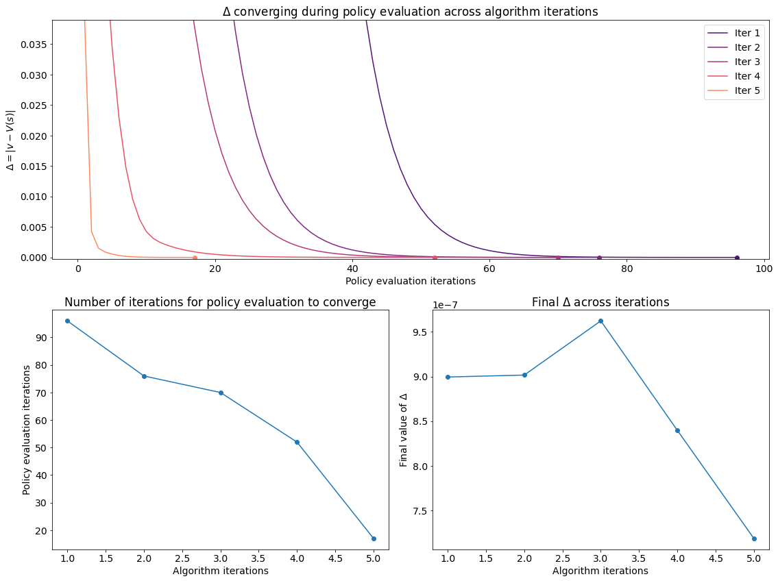
Iteration 1, Policy Eval Iteration 96, Δ = 8.99483e-07
Policy Evaluation done

Starting Policy Iteration
Policy changed - repeating eval

----------------------------------------------------------------------------------------------------
Starting Policy Evaluation
Iteration 2, Policy Eval Iteration 76, Δ = 9.01651e-07
Policy Evaluation done

Starting Policy Iteration
Policy changed - repeating eval

----------------------------------------------------------------------------------------------------
Starting Policy Evaluation
Iteration 3, Policy Eval Iteration 70, Δ = 9.62239e-07
Policy Evaluation done

Starting Policy Iteration
Policy changed - repeating eval

----------------------------------------------------------------------------------------------------
Starting Policy Evaluation
Iteration 4, Policy Eval Iteration 52, Δ = 8.39798e-07
Policy Evaluation done

Starting Policy Iteration
Policy changed - repeating eval

----------------------------------------------------------------------------------------------------
Starting Policy Evaluation
Iteration 5, Policy Eval Iteration 17, Δ = 7.18887e-07
Policy Evaluation done

Starting Policy Iteration
Done
We can visualise the progress of the algorithm in the plots below. Evidently policy evaluation converges faster across iterations of the algorithm and after the first few iterations attains a lower final value.

Visualising the results
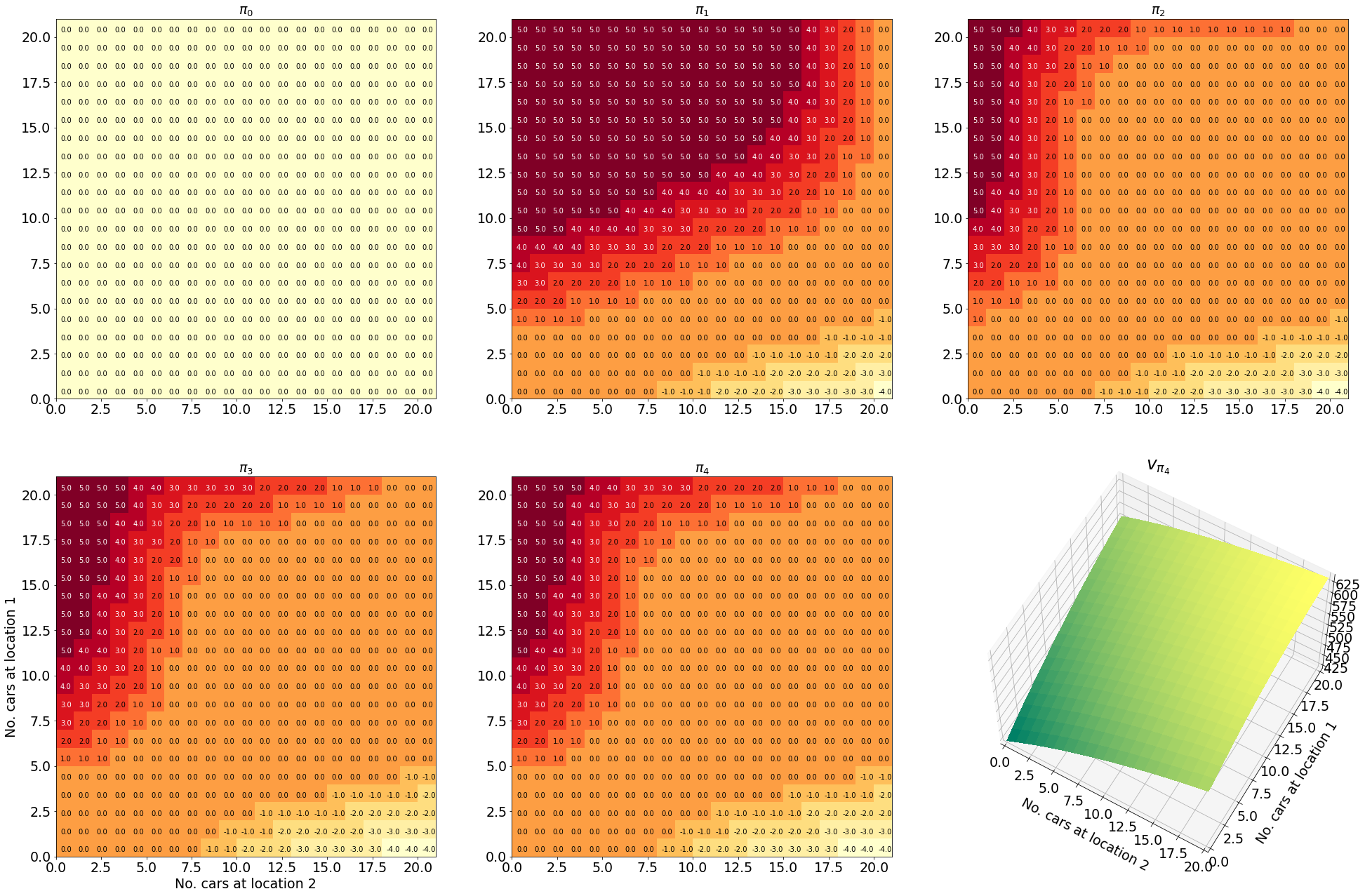
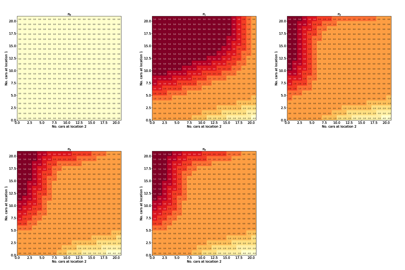
Having successfully run the algorithm, let us visualise the results by creating a figure similar to Figure 4.2 in the RL book. The figure shows the initial policy $\pi_0$ and the policy after each iteration as a heatmap for each combination of the number of cars at each location, $(s_1, s_2)$. It also shows the value function $v_{\pi_4}$ as a 3D plot for each state.
The policies are in a flattened form so we reshape them into a 2D grid for plotting the results in the form of heatmaps. We also reshape the states and values into 21x21
pi_grid = np.reshape([pi[i] for i in state_idx], (21, 21))
idx_grid = np.reshape([states[i] for i in state_idx], (21, 21, 2))
V_grid = np.reshape([V[i] for i in state_idx], (21, 21))
Here is a helper function that adds text labels to the grid. The function takes the states, values, mask and offsets for the text labels as arguments. It also takes a threshold and a boolean lower which determines whether the mask is applied to values lower or higher than the threshold. The function then plots the values as text on the grid, with the text colour set to white if the mask is satisfied and black otherwise.
def plot_grid(states, values, mask, offx, offy, th, axis=None, lower=True):
    # Assumes a colormesh has already been plotted on the axis
    # and adds text labels to the grid
    axis = plt.gca() if axis is None else axis
    for state, value, m in zip(states, values, mask):
        axis.text(state[1]+offx,state[0]+offy,value,
                 color='white' if (m < th if lower else m > th) else 'k')
Finally let us make the plots. The plots are arranged in a 2x3 grid. The first 5 plots show the policies $\pi_0, \pi_1, \pi_2, \pi_3, \pi_4$ and the last plot shows the value function $v_{\pi_4}$.
fig = plt.figure(figsize=(33, 22))

gs = plt.GridSpec(2, 3)
fontsize = 19

cmap = 'YlOrRd'

for t in range(len(history) + 1):


    if t < 5:
        pi_grid_i = np.reshape([history[t][i] for i in state_idx], (21, 21))
        axis = plt.subplot(gs[t])
        axis.pcolormesh(pi_grid_i, cmap=cmap)

        plot_grid(
            idx_grid.reshape([-1, 2]),
            pi_grid_i.reshape([-1]),
            pi_grid_i.reshape([-1]),
            .25, .25, 2, axis=axis, lower=False
        )
        axis.set_aspect('equal', adjustable='box')
        axis.set_title(f'$\pi_{t}$', fontsize=fontsize)

    else:
        axis = plt.subplot(gs[-1], projection='3d')
        X = idx_grid[..., 1]
        Y = idx_grid[..., 0]
        Z = V_grid
        axis.plot_surface(X, Y, Z, cmap='summer', linewidth=0, antialiased=False)
        axis.view_init(60, -60)
        axis.set_xlim([0, 20])
        axis.set_ylim([0, 20]);
        axis.set_title('$v_{\\pi_4}$', fontsize=25)

    if t in [3, 5]:
        space = '\n'*2 if t == 5 else ''
        axis.set_ylabel(f'{space}No. cars at location 1', fontsize=fontsize)
        axis.set_xlabel(f'{space}No. cars at location 2', fontsize=fontsize)

    axis.tick_params(labelsize=fontsize)

Here is an animated version showing how the algorithm progresses towards the final result

And here is an interactive version of the final state-value function