In this post we will introduce the key hyperparameters involved in cosine decay and take a look at how the decay part can be achieved in TensorFlow and PyTorch. In a subsequent blog we will look at how to add restarts.
Cosine Learning Rate Decay
A cosine learning rate decay schedule drops the learning rate in such a way it has the form of a sinusoid. Typically it is used with “restarts” where once the learning rate reaches a minimum value it is increased to a maximum value again (which might be different from the original max value) and it is decayed again.
import torch
import tensorflow as tf
import numpy as np
Basics
The equation for decay as stated in SGDR: Stochastic Gradient Descent with Warm Restarts is as follows
\[\eta_t = \eta^i_{\min} + \frac{1}{2}(\eta^i_{\max} - \eta^i_{\min})\left(1 + \cos\left(\frac{T^i_\text{cur}\pi}{T^i}\right)\right)\]where $i$ means the $i$-th run of the decay. Here will consider a single such run.
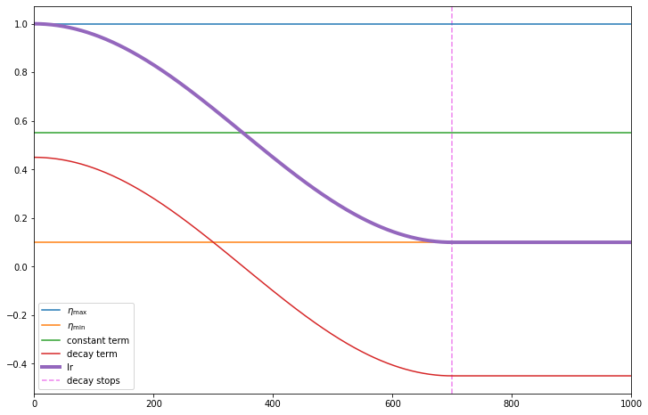
The equation can be expanded (dropping the $i$ superscript) as the sum of a constant and a term that decays over the period $T$ and denoting $T_\text{cur}$ as $t$.
\[\eta_t = \frac{1}{2}(\eta_{\max} + \eta_{\min}) + \frac{1}{2}(\eta_{\max} - \eta_{\min}) \cos\left(\frac{t\pi}{T}\right)\]TensorFlow
In TensorFlow this is implemented by
tf.keras.optimizers.schedules.CosineDecay(
    initial_learning_rate, decay_steps, alpha=0.0, name=None
)
initial_learning_rate= $\eta_{\max}$alpha= $\eta_{\min} / \eta_{\max}$decay_steps= $T$
eta_max = 1.
eta_min =0.1
T = 700
iters = np.linspace(0, 1000,1001)
cos_decay_tf = tf.keras.experimental.CosineDecay(initial_learning_rate=eta_max,
                                                alpha=eta_min/eta_max, decay_steps=T)
import matplotlib.pyplot as plt
plt.figure(figsize=(12, 8))
eta_max = 1
eta_min =0.1
const_term = (eta_max + eta_min) / 2
lr_tf = cos_decay_tf(iters)
ax = plt.axes()
plt.plot(iters, eta_max * np.ones_like(iters), label='$\eta_{\max}$')
plt.plot(iters, eta_min * np.ones_like(iters), label='$\eta_{\min}$')
plt.plot(iters, const_term  * np.ones_like(iters), label='constant term')
plt.plot(iters, lr_tf - const_term, label='decay term')
plt.plot(iters, lr_tf , label='lr', linewidth=4);
ylim = ax.get_ylim()
plt.vlines(x=T, ymin=ylim[0], ymax=ylim[1], linestyle='--', color='violet', label='decay stops')
plt.legend();
plt.xlim(0, np.max(iters))
plt.ylim(ylim);
PyTorch
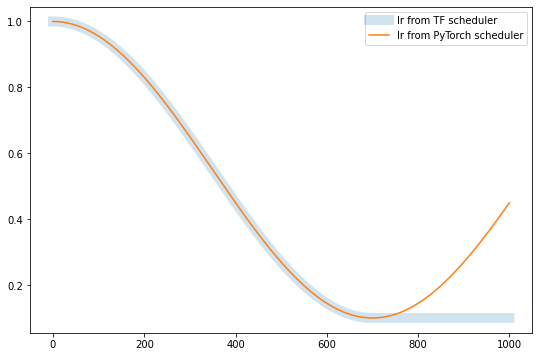
In the PyTorch implementation there are some additional arguments that are relevant for when the learning rate is not solely determined by this schedule which we won’t consider here (see documentation). We will consider the case where the learning rate is dropped by cosine decay alone. A key difference with this implementation is that the learning rate is not clamped to $\eta_{\min}$ after $T$ steps but continues to oscillate.
torch.optim.lr_scheduler.CosineAnnealingLR(optimizer, T_max, eta_min=0, last_epoch=-1, verbose=False)
eta_min= $\eta_{\min}$T_max= $T$
Note that $\eta_{\max}$ is not given to the scheduler but is obtained via the optimizer with which the scheduler must be initialised.
sgd_torch = torch.optim.SGD(lr=1., params=[torch.Tensor()])
sgd_torch.param_groups[0]['initial_lr'] = 1
cos_lr = torch.optim.lr_scheduler.CosineAnnealingLR(sgd_torch, T_max=T, eta_min=0.1)
In this simple example there is a single parameter group and the learning rate can be accessed as sgd_torch.param_groups[0]['lr']. To update the learning rate we take an optimisation step followed by a scheduler step. Also note that we have assigned lr for step 0 so we start at step 1 onwards.
lr_torch = [sgd_torch.param_groups[0]['lr']]
for t in iters[1:]:
    sgd_torch.step()
    cos_lr.step()
    lr_torch.append(sgd_torch.param_groups[0]['lr'])
plt.figure(figsize=(9, 6))
plt.plot(iters, lr_tf, linewidth=10, alpha=0.2, label='lr from TF scheduler')
plt.plot(iters, lr_torch, label='lr from PyTorch scheduler')
plt.legend();
# Steps 0...700
np.allclose(lr_tf[:701], lr_torch[:701])
True
sgd_torch = torch.optim.SGD(lr=1., params=[torch.Tensor()])
sgd_torch.param_groups[0]['initial_lr'] = 1
cos_lr = torch.optim.lr_scheduler.CosineAnnealingLR(sgd_torch, T_max=T, eta_min=0.1)

lr_torch_clamp = [sgd_torch.param_groups[0]['lr']]
for t in iters[1:]:
    sgd_torch.step()
    if t <= T:
        cos_lr.step()
    lr_torch_clamp.append(sgd_torch.param_groups[0]['lr'])
plt.figure(figsize=(9, 6))
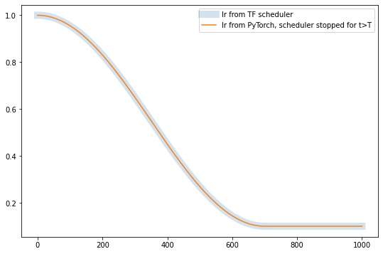
plt.plot(iters, lr_tf, linewidth=10, alpha=0.2, label='lr from TF scheduler')
plt.plot(iters, lr_torch_clamp, label='lr from PyTorch, scheduler stopped for t>T')
plt.legend();
# All steps
np.allclose(lr_tf, lr_torch_clamp)
True
What’s next
Next time will learn how to add warm restarts.