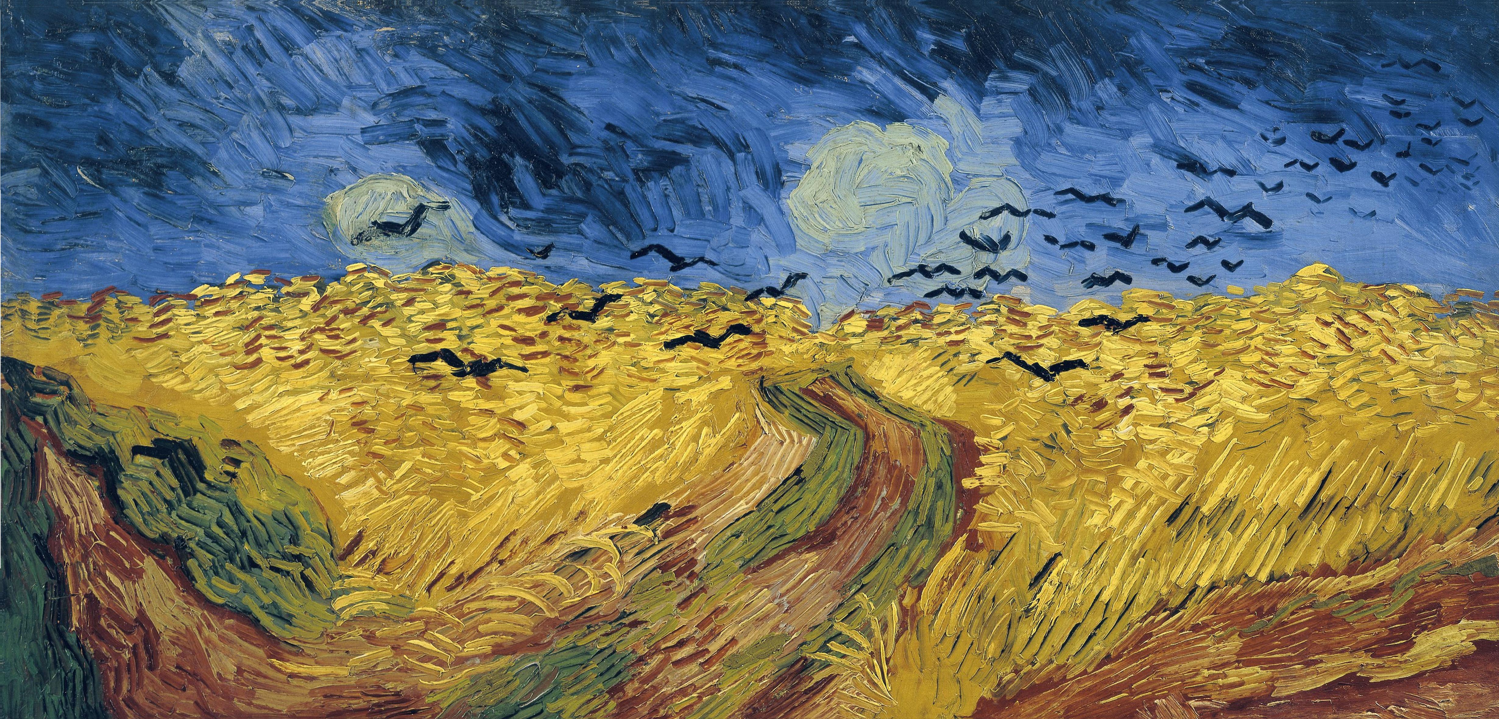
Consider this painting by Vincent Van Gogh known as “Wheatfield with Crows”. Suppose you want to learn a probability distribution over Van Gogh’s paintings. What the computer or a deep learning algorithm sees when it looks at this painting is a grid of RGB pixel intensities. So one approach might be to model the data as a sequence of individual pixels. Yet that is manifestly not how the artist has constructed the painting.
If we knew the sequence of brush strokes made by Van Gogh we could represent the image more concisely in terms of this sequence. A brush stroke might have starting point and an endpoint and properties like color, thickness, opacity, etc and we could write an algorithm that fills in pixels in a grid according to this pattern. Since there are far fewer brush strokes than pixels this would give us a more concise representation of the painting.
An even briefer and perhaps more meaningful representation would be merely to describe what it depicts and how. Two examples:
- Merely what the title states “Wheatfield with Crows”
-
A more detailed description of the content and style:
[A] dramatic, cloudy sky filled with crows over a wheat field. [1]
The blue sky contrasts with the yellow-orange corn, while the red of the path is enhanced by green strips of grass. [2]
Data and latents
What we have been considering is the processs of generating some data and we have identified a couple of intermediate representations of the data such as a sequence of brush strokes, the things represented in the image.
More formally we have some data $\mathbf{x}$ and posit that there is a latent variable $\mathbf{z}$ underlying the process by which the data is generated. Although the data might be complex and high dimensional a simpler process might be going on behind the scenes that can be described by lower dimensional variables.
In the example we have some notion of how the painting was generated based on how a picture is painted and more generally our knowledge of Van Gogh’s methods and ideas. But typically we will not make any assumptions about the structure of the latent space beyond assuming that it is lower dimensional compared to the data.
A generative model
We start with the following ingredients
- Data $\mathbf{x}$ from our dataset which is considered a random variable
- Latent random variables $\mathbf{z}$
- A prior distribution $p_Z(\mathbf{z})$ over $\mathbf{z}$ which can be assumed e.g. $\mathbf{z} \sim \mathcal{N}(0, I)$ or learned.
The goal is to learn a distribution $p_\theta(\mathbf{x} \vert \mathbf{z})$ with parameters $\theta$ which is typically represented by a neural network. This will let us sample from it as follows:
\[z \sim p(\mathbf{x}) \\ x \sim p_\theta(\mathbf{x} \vert \mathbf{z})\]We would like to train it by optimising the log likelihood over a batch of examples $\mathbf{x}^{(i)}$
\[\max_\theta \sum_i \log p_\theta\left(\mathbf{x}^{(i)}\right) = \sum_i \log \sum_z p_Z(\mathbf{z})p_\theta\left(\mathbf{x}^{(i)}\vert \mathbf{z}\right)\]We also want to be able to estimate $z$ from $x$. Ideally we could use Bayes rule to go from data to latents:
\[p_\theta( \mathbf{z}\vert \mathbf{x}) = \frac{p_\theta(\mathbf{x} \vert \mathbf{z})p_Z(\mathbf{z})}{p_\theta (\mathbf{x})}\]If $\mathbf{z}$ is continuous valued \(p_\theta (\mathbf{x}) = \int_Z p_\theta(\mathbf{x} \vert \mathbf{z})p_Z(\mathbf{z}) d\mathbf{z}\)
For discrete $\mathbf{z}$
\[p_\theta (\mathbf{x}) = \sum_{\mathbf{z} \in Z} p_\theta(\mathbf{x} \vert \mathbf{z})p_Z(\mathbf{z}) d\mathbf{z}\]The problem is evaluating $p_\theta (\mathbf{x})$ for arbitrary latent spaces. If $\mathbf{z}$ only takes on a limited number of values or if it is possible to evaluate the integral then it can be calculated exactly.
In general this is not the case. Instead we pick a distribution $q_\phi(\mathbf{z} \vert \mathbf{x})$ with parameters $\phi$ and optimise the parameters until it becomes close to the true conditional distribution. The model then looks like this:

We then jointly train models for $p_\theta$ and $q_\phi$ to minimise the following loss function which comprises the negative KL-divergence between the $q_\phi(\mathbf{z} \vert \mathbf{x})$ and the prior over $\mathbf{z}$, and the expected value of the log-likelihood
\[L(\theta, \phi) = -D_{KL}\left( q_\phi(\mathbf{z} \vert \mathbf{x})\Vert p_\theta(\mathbf{z})\right) + \mathbb{E}_{q_\phi(\mathbf{z} \vert \mathbf{x})} \left[\log p_\theta(\mathbf{z}\vert \mathbf{x}) \right]\]What’s next
In the next post we will implement a simple model to get a better sense of the concepts involved. We will then go on to learn how the mathematical ideas behind the VAE.