Introduction
In the previous post we motivated the idea of a Variational Auto Encoder. Here we will have a go at implementing a very simple model to get a sense of all the components steps involved.
This is quite a long post but much of it is just code. All the code in this post can be found in this Colab notebook.
import torch
import math
from torch import nn
import tqdm.notebook as tqdm
from easydict import EasyDict
Data
Here is a simple 2d data distribution
\[\mathbf{x} = \left[x_1, x_2\right]^T\] \[\mathbf{x} \sim N(\mu, \Sigma)\]where $\Sigma$ is a full covariance matrix, meaning that it can have non-zero off-diagonal entries.
import numpy as np
import matplotlib.pyplot as plt

mu = np.stack([1., 0.5])
cov = np.stack([[1, 0.5],
              [0.5, 1]])

import numpy as np

def is_pos_def(x):
    return np.all(np.linalg.eigvals(x) > 0)

assert is_pos_def(cov)

x = np.random.multivariate_normal(
    mu, cov,
    size=10000
)
plt.figure(figsize=(8, 8))
plt.hist2d(x[:, 0], x[:, 1], bins=100, cmap='Blues');
plt.title('samples $\mathbf{x}^{(i)} \sim N(\mu, \Sigma)$');
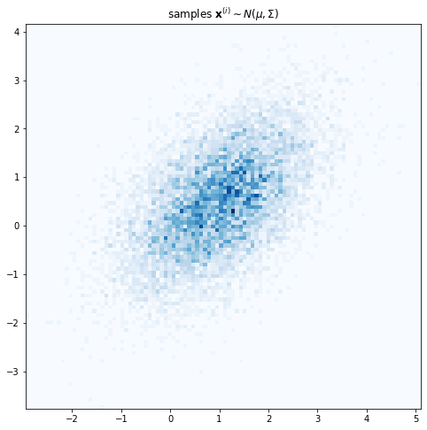
However we assume that conditioned on the latent variable $z$, $\mathbf{x}$ has a simpler diagonal covariance, in other words that $x_1$ and $x_2$ are independent conditioned on $z$.
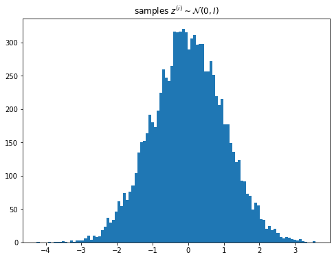
\[\mathbf{z} \sim \mathcal{N}(0, I)\] \[\mathbf{x} \sim \mathcal{N}(\boldsymbol{\mu}, \text{diag}(\boldsymbol{\sigma})))\]plt.figure(figsize=(8, 6))
plt.hist(np.random.normal(size=[10000]), bins=100)
plt.title('samples $z^{(i)} \sim \mathcal{N}(0, I)$');
For $q(\mathbf{z} \vert \theta)$ we choose a normal distribution with a diagonal covariance which means the KL-divergence term in the loss can be found exactly.
Neural network representation
We will use a simple feed-forward network to represent each of $ \mathcal{N}(\mu’, \sigma’^2I \vert \mathbf{z})$ and $q(\mathbf{z} \vert \theta)$. This is the formulation from the VAE paper where the parameters are obtained via 2-layer MLP. Note that the log of the variance is predicted which keeps the output within a smaller range of values compared to predicting the raw variance.
\[\log p_{\theta}\left (\mathbf{x} \vert \mathbf{z} \right) = \log \mathcal{N}(\mu, \sigma^2I \vert \mathbf{z})\] \[\mathbf{h} = \text{Dense}(\mathbf{x})\] \[\left[\log \sigma^2;\mu\right] = \text{Dense}(\tanh(\mathbf{h}))\]Similarly for $\mathbf{z}$
\[\log q_{\phi}\left(\mathbf{z} \vert \mathbf{x} \right) = \log \mathcal{N}(\mu, \sigma^2I \vert \mathbf{x})\] \[\mathbf{h} = \text{Dense}(\mathbf{x})\] \[\left[\log \sigma^2;\mu\right] = \text{Dense}(\tanh(\mathbf{h}))\]class GaussianMLP(nn.Module):
def __init__(self, input_dim, hidden_dim, latent_dim):
super(GaussianMLP, self).__init__()
self.shared = nn.Sequential(
nn.Linear(in_features=input_dim,
out_features=hidden_dim),
nn.Tanh()
)
self.param_layer = nn.Linear(in_features=hidden_dim,
out_features=latent_dim * 2)
def forward(self, inputs):
shared = self.shared(inputs)
params = self.param_layer(shared)
return params
First let us create a model comprising these two distributions where $p_{\theta}\left (\mathbf{x} \vert \mathbf{z} \right)$ is called encoder and $q_{\phi}\left(\mathbf{z} \vert \mathbf{x} \right)$ is called decoder.
class VAE(nn.Module):
    def __init__(self, encoder, decoder):
        super(VAE, self).__init__()
        self.encoder=encoder
        self.decoder=decoder
Now let us add functions to run the encoding
def encode(self, inputs):
    params_z = self.encoder(inputs)
    mu_z = params_z[:, :(params_z.size(1)//2)]
    log_sig2_z = params_z[:, (params_z.size(1)//2):]
    return mu_z, log_sig2_z

VAE.encode = encode
And decoding
def decode(self, latents):
    params_x = self.decoder(latents)
    mu_x = params_x[:, :(params_x.size(1)//2)]
    log_sig2_x = params_x[:, (params_x.size(1)//2):]
    return mu_x, log_sig2_x

VAE.decode = decode
Training
- Sample training examples from the ground truth distribution $\mathbf{x}^{(i)} \sim p(\mathbf{x})$
- Predict parameters for $q_\phi(\mathbf{z} \vert \mathbf{x})$
- Sample latents from the approximate distribtion $\mathbf{z}^{(i)} \sim q_\phi(\mathbf{z} \vert \theta)$
- Predict parameters for $p_\theta(\mathbf{x} \vert \mathbf{z})$
- Calculate the loss and run backward pass
Since we are predicting the parameters of a distribution, to calculate the loss we don’t need to sample from $p_\theta(\mathbf{x} \vert \mathbf{z})$. We only need to find the pdf of the distribution which can be done e.g. via torch.distributions.Normal.
def forward(self, inputs, noise):
        # inputs: [B, H, W, F]
        # noise: [N, B, Z]
        mu_z, log_sig2_z = self.encode(inputs)
        # [N, B, Z]
        latents = sample_latents(mu_z, log_sig2_z, noise)
        # [N * B, Z]
        mu_x, log_sig_x = self.decode(latents.reshape(-1, latents.size(-1)))
        # [N, B, Z], [B, Z], [B, Z], [N, B, H, W, F]
        return (latents, mu_z, log_sig2_z,
                mu_x.reshape(-1, *inputs.size()),
                log_sig_x.reshape(-1, *inputs.size()))
VAE.forward = forward
Reparameterization Trick
Now at this point you might have some questions
- Where did this
noisecome from? - What is the
sample_latentsfunction doing?
Now we will go into more details about the mathematics behind all this in a subsequent post (coming soon) but in simple terms consider this diagram of the steps involved. Remember that for the loss here we don’t need to sample from $p_\theta(\mathbf{x} \vert \mathbf{z})$ so the graph stops after predicting the parameters of this distribution.
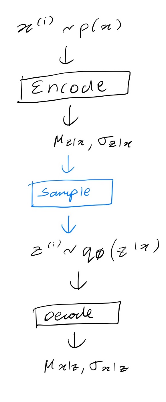
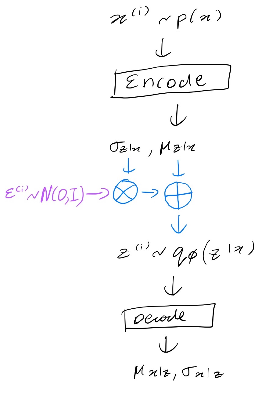
We can’t differentiate through the sampling step shown in blue. To get around that the authors of the paper use a reparameterization trick whereby you generate noise samples $\mathbf{\epsilon^{(i)}}$ e.g. from $\mathcal{N}(0, I)$, transform them to $\mathbf{z}^{(i)}$ and input these to the decoder. The transformation is done in a differentiable way. For a normal distribution you can convert samples $\boldsymbol{\epsilon} \sim \mathcal{N}(0, I)$ to samples $\mathbf{z}^{(i)} \sim \mathcal{N}(\boldsymbol{\mu}, \text{diag}(\boldsymbol{\sigma})))$ by transforming each element $z_i$ as follows
\[z_i = \sigma_i \cdot \epsilon_i + \mu_i\]Now we can differentiate through the blue part in the figure below.
The sample_latents functions simply transforms the noise into latents.
def sample_latents(mu, log_var, noise):
    return mu + torch.exp(log_var / 2) * noise
Loss
Finally let us add a loss function that calls forward and then calculates the loss given by this expression we saw earlier.
Often we can’t calculate this exactly so we have to approximate it. For the log likelihood term the approximation is as follows for a single $\mathbf{x}^{(i)}$:
\[\mathbb{E}_{q_\phi(\mathbf{z} \vert \mathbf{x}^{(i)})} \left[\log p_\theta(\mathbf{z}\vert \mathbf{x}^{(i)}) \right] \approx \frac{1}{T}\sum_{t=1}^T\log p_\theta(\mathbf{x}^{(i)} \vert \mathbf{z}^{(i, t)})\]You might have noted that the noise input has shape [N, B, Z]. That is because we sample an $\boldsymbol{\epsilon}^{(i, t)}$ corresponding to each $\mathbf{z}^{(i, t)}$.
It turns out that because both $p_\theta$ and $q_\phi$ are normal distributions, the KL divergence term becomes a simple expression that can be calculated exactly. Here is the expression for a $J$ dimensional latent
\[-D_{KL}\left( q_\phi(\mathbf{z} \vert \mathbf{x}^{(i)})\Vert p_\theta(\mathbf{z})\right) = \frac{1}{2}\sum_{j=1}^J\left(1 + \log((\sigma_j^{(i)})^2) - (\mu_j^{(i)})^2 - (\sigma_j^{(i)})^2\right)\]We derive all of this in a future post.
def loss(self, x, noise):
        z, mu_z, log_sig2_z, mu_x, log_sig2_x = self(x, noise)
        KL = -(1 + log_sig2_z - mu_z**2 - torch.exp(log_sig2_z)) / 2
        KL_term = KL.sum(dim=-1).mean()
        recon = -torch.distributions.Normal(mu_x, torch.exp(log_sig2_x/2)).log_prob(x)
        recon = recon.sum(dim=-1).mean()
        return KL_term + recon, recon, KL_term

VAE.loss = loss
Now we can combine all these parts into a training step
def train_step(cfg, vae, optim, batch):
    optim.zero_grad()
    noise = torch.randn([cfg.num_mc, batch.size(0), cfg.latent_dim])
    loss, recon_loss, KL_term = vae.loss(batch, noise)
    loss.backward()
    optim.step()
    return loss.detach().numpy(), KL_term.detach().numpy(), recon_loss.detach().numpy()
We can write a similar function to calculate losses during validation. Here we use the same noise values each time.
def run_test(data, model, batch_size, latent_size, num_mc, noise):
    # noise: [T, N, B, L]
    model.eval()
    num_iters = math.ceil(len(data) / batch_size)
    losses = []
    counts = []
    for idx in tqdm.trange(num_iters):
        slc = slice(idx * batch_size, (idx + 1) * batch_size)
        batch = torch.from_numpy(data[slc])
        loss = model.loss(batch, noise[idx, :, :batch.size(0)])
        losses.append([l.detach().numpy() for l in loss])
        counts.append(len(batch))
    return np.sum(losses * np.stack(counts)[:, None], axis=0) / np.sum(counts)
Inference
- Sample latents from the prior $z^{(i)} \sim \mathcal{N}(0, I)$
- Predict parameters for $p_\theta(\mathbf{x} \vert \mathbf{z})$
- Sample from $p_\theta(\mathbf{x} \vert \mathbf{z})$
Note we might also just choose to return $\mu_{\mathbf{x}\vert\mathbf{z}}$ instead of sampling from $p_\theta(\mathbf{x} \vert \mathbf{z})$. This tends to be the case when dealing with high dimensional data like images where the samples tend be too noisy.
def generate_samples(cfg, vae, n_samples, noise=False):
    vae.eval()
    with torch.no_grad():
        z = torch.randn([n_samples, cfg.latent_dim])
        mu_x, log_sig_x = vae.decode(z)


        if noise:
            # 1 sample per latent
            return torch.distributions.Normal(mu_x, torch.exp(log_sig_x /2)).sample().cpu().numpy()

    return mu_x.cpu().numpy()
Putting it together
Let us write a run_model function that sets up the models and goes through all the steps described above.
def run_model(cfg, train_data, test_data):

    # Initialise encoder and decoder
    encoder = GaussianMLP(input_dim=cfg.input_dim,
                               hidden_dim=cfg.hidden_dim,
                               latent_dim=cfg.latent_dim,
                               )
    decoder = GaussianMLP(input_dim=cfg.latent_dim,
                               hidden_dim=cfg.hidden_dim,
                               latent_dim=cfg.input_dim,
                               )

    # Initialise VAE
    vae = VAE(encoder, decoder)

    # Intialise optimizer
    optim = torch.optim.Adam(params=vae.parameters(), lr=1e-3)

    # Initialise other values and data structures
    batch_size = cfg.batch_size

    num_train_iters = math.ceil(len(train_data) / batch_size)


    train_losses, test_losses, num = [], [], []

    train_data = train_data
    test_data = test_data

    # Noise to be reused for testing
    noise_val = torch.randn(
        [math.ceil(len(test_data) / batch_size),
         cfg.num_mc, batch_size, cfg.latent_dim]
    )

    # Run a forward pass on the uninitialised model
    test_losses.append(run_test(test_data, vae, batch_size, cfg.latent_dim, cfg.num_mc, noise_val))

    print(f"Initial Test loss: {test_losses[-1][0]:.4f}")

    # For visualisation we might want to save samples after each step
    if cfg.sample_each_step:
        samples_per_step = []


    for epoch in range(cfg.num_epochs):
        vae.train()

        # Shuffle data each epoch
        train_data = train_data[np.random.permutation(len(train_data))]


        # Train the model for each batch, saving losses and if sample_each_step is True, samples
        for i_trn in tqdm.trange(num_train_iters):
            slc = slice(i_trn * batch_size, (i_trn + 1) * batch_size)
            batch = torch.from_numpy(train_data[slc])
            losses = train_step(cfg, vae, optim, batch)
            train_losses.append(losses)
            num.append(batch.size(0))
            if cfg.sample_each_step:
                samples_per_step.append(generate_samples(cfg, vae, n_samples=cfg.n_samples, noise=True))

        # Run validation
        test_losses.append(run_test(test_data, vae, batch_size, cfg.latent_dim, cfg.num_mc, noise_val))

        print(
            f"Epoch {epoch}",
            f"Training loss: {np.sum([l[0] * b for l, b in zip(train_losses[-num_train_iters:], num[-num_train_iters:])] / np.sum(num[-num_train_iters:]) ):.4f},",
            f"Test loss: {test_losses[-1][0]:.4f}"
        )

    # Generate some samples with and without noise
    samples_no_noise = generate_samples(cfg, vae, n_samples=cfg.n_samples, noise=False)
    samples_with_noise = generate_samples(cfg, vae, n_samples=cfg.n_samples, noise=True)
    result = (np.stack(train_losses), np.stack(test_losses),  samples_with_noise, samples_no_noise)
    return result + (samples_per_step,) if cfg.sample_each_step else result
Now get hold of a bunch of samples.
dataset = np.random.multivariate_normal(
    np.array(mu),
    np.array(cov),
    size=12500,
).astype('float32')

trn_data, tst_data = np.split(dataset, [10000])
Define a few settings
config = EasyDict(
        input_dim=2,
        num_mc=1,
        print_interval=100,
        batch_size=128,
        hidden_dim=512,
        latent_dim=2,
        n_samples=1000,
        num_epochs=1,
        sample_each_step=True
    )
Finally we are ready to run
result = run_model(config, trn_data, tst_data)
Visualising the results
from scipy.stats import multivariate_normal
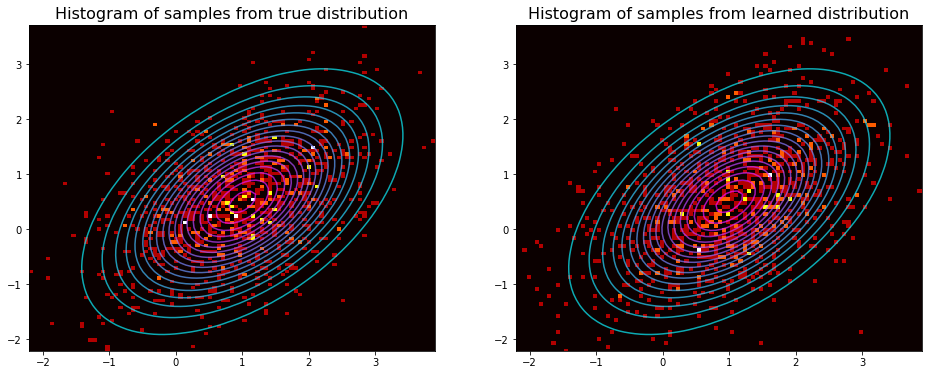
Let us generate some samples from the true distribution and also plot the contours of the probability density function.
mvn = multivariate_normal(mu, cov)
fig, axes = plt.subplots(1, 2, figsize=(16, 6))
xx, yy = np.meshgrid(np.linspace(-3, 5, 100), np.linspace(-3, 7, 100))
p = mvn.pdf(np.stack([xx, yy], axis=-1))

true_data = tst_data[:len(result[-3])]
pred_data = result[-1][-3]
for vals, clr, ax, dist in zip([true_data, pred_data], ['blue', 'purple'], axes, ['true', 'learned']):
    ax.contour(xx, yy, p, levels=20, alpha=0.7, cmap='cool')
    ax.hist2d(*vals.T, bins=100, cmap='hot') #, marker='.', c=clr, alpha=0.5)
    ax.set_title(f'Histogram of samples from {dist} distribution', fontsize=16)
    ax.set_xlim(max(true_data[:, 0].min(), pred_data[:, 0].min()),
                min(true_data[:, 0].max(), pred_data[:, 0].max()),
               )
    ax.set_ylim(max(true_data[:, 1].min(), pred_data[:, 1].min()),
                min(true_data[:, 1].max(), pred_data[:, 1].max()))
Using the saved samples from each step we can see how the model improves over time.
fig, axes = plt.subplots(4, 4, figsize=(16, 16))
xx, yy = np.meshgrid(np.linspace(-3, 5, 100), np.linspace(-3, 7, 100))
p = mvn.pdf(np.stack([xx, yy], axis=-1))
N = 15
size = len(result[-1])
stride = size // N

ax = axes[0, 0]
#cmap = plt.cm.viridis
#ax.contour(xx, yy, p, levels=20,  alpha=0.5, cmap=cmap)
ax.scatter(*tst_data.T,  marker='.', alpha=.8)
ax.set_title(f'True', fontsize=16)
ax.set_xlim(-4, 6)
ax.set_ylim(-4, 5)

for ax, idx, vals in zip(axes.ravel()[1:], np.arange(size)[::stride][:N],
                                     result[-1][::stride][:N]):
    #ax.contour(xx, yy, p, levels=20,  alpha=0.5, cmap=cmap)
    ax.scatter(*vals.T, c='green', marker='.', alpha=.8)
    ax.set_title(f'Generated / step {idx + 1}', fontsize=16)
    ax.set_xlim(-4, 6)
    ax.set_ylim(-4, 5)
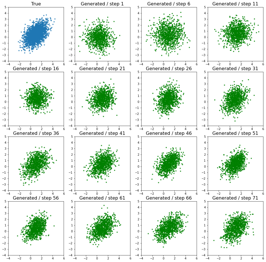
This is a simple task and it can be seen that the model is very quickly able to learn the distribution
What’s next
In the subsequent blog posts we will start delving into the mathematical details that we only briefly mentioned here. We will also learn how to implement more sophisticated VAEs.