import numpy as np
import matplotlib.pyplot as plt
import sys
In this blog post we will reproduce Examples 3.5 and 3.8 in Reinforcement Learning (Sutton and Barto) involving the Bellman equation. This post presumes a basic understanding of reinforcement learning in particular policy and value and will just outline the theory that is needed in order to implement the examples. For more details please refer to chapters 3 and 4 of Sutton and Barto.
\(\newcommand{\sb}[2]{\text{}{#1}_{#2}\text{}}\) \(\newcommand{\sixstar}{*}\)
Theory
The basic idea is that you have an agent that interacts with an environment by choosing and taking actions $a$ which result in rewards $r$ that it seeks to maximise over time. The state $s$ is a representation of the environment that the agent receives at each time step based on which it decides how to act resulting in a sequence of the form state->action->reward->next_state->…
For Markov decision processes the value of a state $s$ under policy $\pi$ is given by
\[v_\pi(s) = \mathbb{E}_\pi[G_t \lvert S_t=s]=\mathbb{E}_\pi\left[\sum\limits_{k=0}^{\infty}\gamma^kR_{t + k + 1} \Bigg\vert S_t = s \right] \forall{s }\in \mathcal{S}\\\]The policy is a distribution over the actions $a$ given a state which indicates how likely an action will be taken from a state
The expected value of the reward from this state is as follows
\[\mathbb{E}_\pi[R_{t+1}\lvert S_t=s] = \sum_{r} r\cdot p(R_{t+1} = r \vert S_t = s)\\ = \sum_{s', r, a} r \cdot p(R_{t+1} = r, S_{t+1} = s' \vert A_t = a, S_t = s)\cdot \pi(A_t = a\vert S_t = s)\]The return at timestep $t$, $G_t$, is defined as the discounted sum of all future rewards starting at $t$:
\[G_{t} = \sum_{z=0}^\infty \gamma^z R_{t + z + 1}\]The expected return following state $s$ at timestep $t$ can be written as
\[\mathbb{E}_\pi[G_{t+1}\lvert S_t=s] = \sum_{s', a} \mathbb{E}_\pi[G_{t+1} \lvert S_{t+1}=s', S_t = s] \cdot p(S_{t+1} = s' | S_t = s, A_t = a)\cdot \pi(A_t = a\vert S_t = s) \\= \sum_{s', a} \mathbb{E}_\pi[G_{t+1} \lvert S_{t+1}=s']\cdot p(S_{t+1} = s' | S_t = s, A_t = a)\cdot \pi(A_t = a\vert S_t = s)\]where the last line comes about since given $S_{t+1}$, $G_{t+1}$ does not depend on $S_t$. Then, plugging in the expression for $v_\pi$ defined earlier we get
\[\mathbb{E}_\pi[G_{t+1}\lvert S_t=s] =\sum_{s', r, a} v_\pi(s')\cdot p(R_{t+1} = r, S_{t+1}=s' \vert S_t = s, A_t = a)\cdot \pi(A_t = a\vert S_t = s)\]Thus we can write the Bellman equation
\[v_\pi(s) = \mathbb{E}_\pi[R_{t+1} + \gamma G_{t+1} \lvert S_t=s] = \sum_a \pi(a\vert s) \sum_{s'}\sum_r p(s', r \vert s, a)\left[r + \gamma v_\pi(s')\right]\]Vectorised form
For $N$ discrete reward values, ${\rho_0, \rho_1, \ldots, \rho_N}$, let be $\boldsymbol{\rho}$ a column vector where $\boldsymbol{\rho}_r = r$. Then assuming that $s = {0, 1, … ,\lvert\mathcal{S}\rvert-1}$ (which can be achieved by mapping each state to an index):
\[\sum_{r} r\sum_{a, s'} p(s', r \vert s, a) \cdot \pi(a\vert s)= \sum_r \boldsymbol{\rho}_r \sum_{a, s'} \pi(a\vert s) \cdot p(s', r \vert s, a) = (\mathbf{Q}\boldsymbol{\rho})_s\] \[\mathbf{Q} \in \mathbb{R}^{N \times |S|}, \text{ }\mathbf{Q}_{rs} = \sum_{a, s'} p(s', r \vert s, a) \cdot \pi(a\vert s)\]Similarly, with $\mathbf{v}$ as a row vector with dimension $\vert S \vert$, where $\mathbf{v}_{s’} = v_\pi(s’)$:
\[\sum_a \pi(a\vert s) \sum_{s', r} \gamma v_\pi(s')\cdot p(s', r \vert s, a) = \gamma\sum_{s'} \mathbf{v}_{s'}\sum_{a, r} p(s', r \vert s, a) \cdot \pi(a\vert s) = \gamma(\mathbf{R}\mathbf{v})_s\] \[\mathbf{R} \in \mathbb{R}^{|S| \times |S|}, \text{ }\mathbf{R}_{s's} = \sum_{a, r} p(s', r \vert s, a) \cdot \pi(a\vert s)\]Putting this together
\[\mathbf{v} = \mathbf{Q}\boldsymbol{\rho} + \gamma\mathbf{R}\mathbf{v}\]Solving for $\mathbf{v}$:
\[(\mathbf{I} - \gamma\mathbf{R})\mathbf{v} = \mathbf{Q}\boldsymbol{\rho} \implies \mathbf{v} = (\mathbf{I} - \gamma\mathbf{R})^{-1}\mathbf{Q}\boldsymbol{\rho}\]Gridworld (Example 3.2)
This is a simple environment where states are positions on a $5 \times 5$ grid
h = w = 5
states = np.stack(np.meshgrid(np.arange(h), np.arange(w))[::-1], axis=-1).reshape((25,2))
# Map rewards to [0, number of state values)
state2ind = dict(zip(map(tuple, states), range(len(states))))
The actions are move one cell up, down, left or right. Here we consider a uniform policy which assigns equal probability for all states. Hence $\pi(a \vert s)$ can be represented by a $4 \times 25$ matrix where every element is 0.25.
actions = np.array([[1,0],[0,1],[-1,0],[0,-1]])
pi = np.tile([[0.25]], [4, 25])
There are two special states $A$ and $B$ where every action leads to a jump to the next states $A’$ and $B’$. For every other state all actions lead to the neighbouring state that depends on the action - unless this action would lead to a state outside the grid in which case the next state is the same as the present state.
state_a = np.array([0,1])
state_b = np.array([0,3])
next_a = np.array([4,1])
next_b = np.array([2,3])
For next states $A’$ the reward is 10 and for $B’$ it is $5$. For all other next states rewards are $0$ unless the action leads to a state outside the grid in which case the reward is $-1$
rewards = np.array([-1,0,5,10])
# Map rewards to [0, number of reward values)
rewards2ind = dict(zip(rewards, range(len(rewards))))
def out_of_bounds(state, h, w):
    return np.logical_or(np.any(state >= [h,w], axis=-1),
                          np.any(state < [0,0], axis=-1))
out_of_bounds(states, h, w)
array([False, False, False, False, False, False, False, False, False,
       False, False, False, False, False, False, False, False, False,
       False, False, False, False, False, False, False])
Note that given the present state $s$ and action $a$, there is a single possible next state and reward which means for this particular $s’, r$, $p(s’,r \vert s, a) = 1$. We will now create a $4D$ tensor for $p(s’,r \vert s, a)$ i.e. at tensor with dimensions $\lvert\mathcal{S}\rvert \times \lvert\mathcal{R}\rvert \times \lvert\mathcal{S}\rvert \times \lvert\mathcal{A}\rvert = 25 \times 4 \times 25 \times 4$. For each $s, a$ this matrix consists of a $\lvert\mathcal{S}\rvert \times \lvert\mathcal{R}\rvert$ tensor that is 1 at the element corresponding to $s’, r’$ and 0 everywhere else
P = np.zeros((states.shape[0], rewards.shape[0], states.shape[0], actions.shape[0]))
for s,state in enumerate(states):

    for a,action in enumerate(actions):
        # Identify the next state and reward
        if np.all(state == state_a):
            next_state = next_a
            reward = 10
        elif np.all(state == state_b):
            next_state = next_b
            reward = 5
        else:
            next_state = state + action

            #Determine if next state is outside the grid boundaries
            if out_of_bounds(next_state, h, w):
                next_state = state
                reward = -1

            else:
                reward = 0

        P[state2ind[tuple(next_state)], rewards2ind[reward], s, a] = 1
# - Sum over s',a, multiply with transposed pi then transpose to get Q
Q = np.einsum('Srsa,as->sr', P, pi)
# - Sum over r,a, multiply with transposed pi then transpose to get R
R = np.einsum('Srsa,as->sS', P, pi)
gamma = 0.9
y = np.einsum('sr,r->s', Q, rewards)
# Note that `S` has the same size as `s` since both are the number of states but `S` corresponds
# to the next state axis whilst `s` to the present state
v = np.einsum('sS,S->s', np.linalg.inv(np.eye(R.shape[0]) - gamma*R), y)
def make_grid(v, shape):
    return v.reshape(shape)
def plot_grid(states, values, offx, offy, th):
    for state, value in zip(states, values):
        plt.text(state[1]+offx,state[0]+offy,np.round(value,1),
                 color='white' if value < th else 'k')
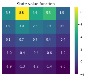
v_grid = make_grid(np.round(v,1),[5,5])
v_grid should be the same as in the diagram shown in the book for Example 3.5 when rounded to 1
v_true = np.array([[ 3.3,  8.8,  4.4,  5.3,  1.5],
                   [ 1.5,  3. ,  2.3,  1.9,  0.5],
                   [ 0.1,  0.7,  0.7,  0.4, -0.4],
                   [-1. , -0.4, -0.4, -0.6, -1.2],
                   [-1.9, -1.3, -1.2, -1.4, -2. ]])
def values_match(v_true, v):
    return np.all(v_true.reshape(-1)==np.round(v,1))
print(values_match(v_true, v))
True
plt.imshow(v_grid)
plt.title('State-value function')
plt.colorbar();
plt.axis('off');
plot_grid(states, v, -0.25, 0, 8)
Optimal value function
The Bellman optimality equation is given as
\[v_*(s) = \max_a \sum_{s',r}p(s', r \lvert s, a)\left[r + \gamma v^*(s')\right]\]Below $\mathbf{P}$ is the $4D$ tensor defined above where $\sb{\mathbf{P}}{s’rsa} = p(s’,r\lvert s, a)$ where $\sb{\mathbf{P}}{s’ : s a}$ is the $\lvert\mathcal{R}\rvert$-d vector obtaining by fixing $s’, s$ and $a$ whilst $\sb{\mathbf{P}}{: r s a}$ is the $\lvert\mathcal{S}\rvert$-d vector obtained by fixing $r, s$ and $a$.
\[\mathbf{v}^*_s = \max_a \left( \sum_{s'}\mathbf{P}_{s' : s a}^T\boldsymbol{\rho} + \gamma\sum_{r}\mathbf{P}_{: r s a}^T\mathbf{v}^* \right)\]Estimating the best policy $\boldsymbol{\pi}^*$ iteratively
This equation for $\sb{\mathbf{v}^\sixstar}{s}$ is not a linear equation so we can’t solve it as before but we can estimate the solution iteratively. We will initialise $\mathbf{v}$ and $\pi$ with some value and keep updating $v$ with the max over all actions $a$ of $\sum_{s’}\sb{\mathbf{P}}{s’ : s a}^T\boldsymbol{\rho} + \gamma\sum_{i}\sb{\mathbf{P}}{: r s a}^T\mathbf{v}^\sixstar$ until the difference between consecutive value functions becomes negligible. The actions at a given state that yield the best value i.e. the argmax of the RHS will then give us the best policy $\pi^\sixstar$.
The method for Iterative Policy Evaluation given in Sutton and Barto
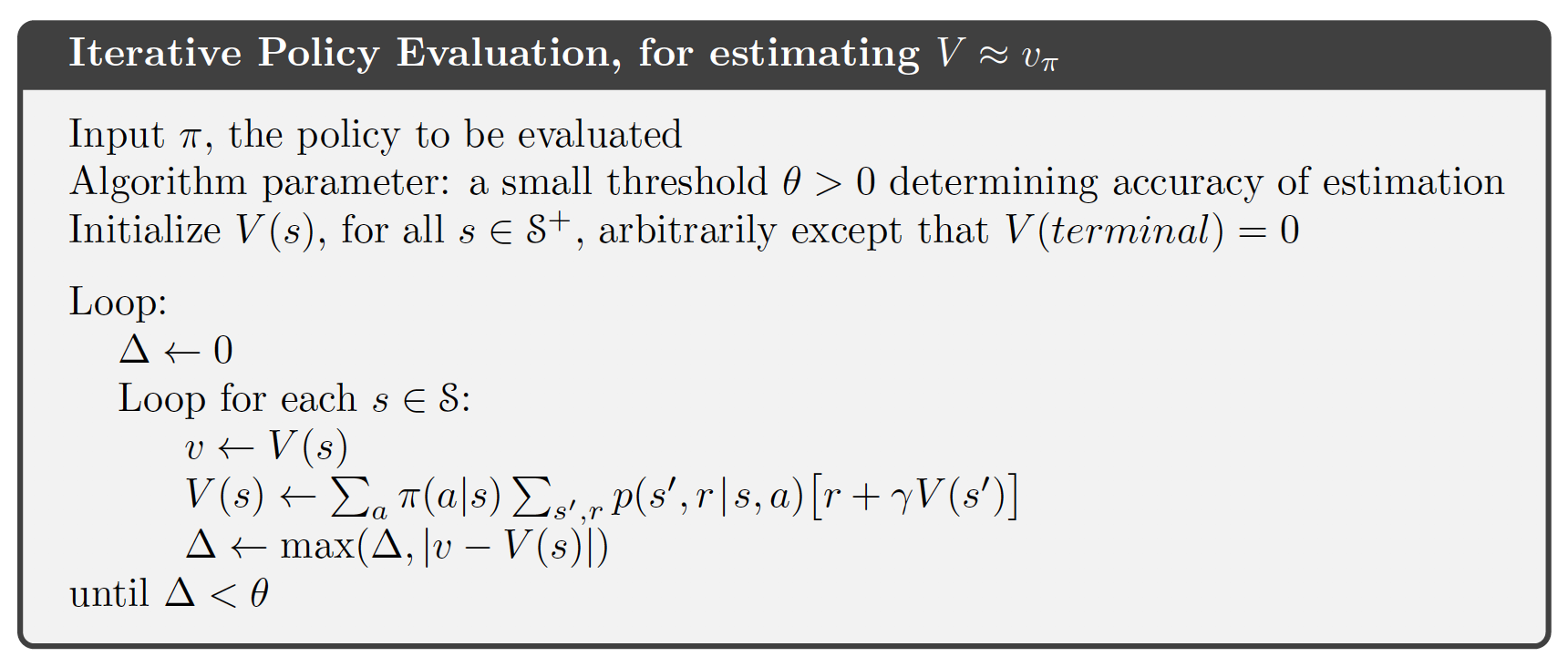
A difference between our implementation and the method above is that we are not doing in place updates since we are using a vectorised approach.
def estimate_vstar(v_init, prob_next_reward, rewards, gamma = 0.9, tol=1e-12):
    iters = 0
    v_prev = v_init
    vs = [v_prev]
    diffs = []
    while True:
        iters+=1
        QQ = np.einsum('Srsa,r->sa', prob_next_reward, rewards)
        RR = np.einsum('Srsa,S->sa',prob_next_reward, v_prev)
        v_next = np.max(QQ + gamma*RR, axis=-1)
        diff = np.square(v_prev-v_next)
        diffs.append(np.mean(diff))
        if iters % 20 == 0:
            print('\rIteration {}, mean squared difference {}'.format(iters, diffs[-1]))
        vs.append(v_next)
        if np.all(diff < tol):
            break
        v_prev = v_next

    print('\rFinal iteration {}, mean squared difference {}'.format(iters, diffs[-1]))
    return v_next, vs, diffs, QQ, RR
Solving the Gridworld (Example 3.8)
We will initialise the states arbitrarily. The only requirement is that terminal states should be initialised with $0$ but there are no terminal states here. For simplicity we will initialise all states as 0 and start off with a uniform policy where each action is considered equally good. Since we are considering the same environment as before, we can reuse tensor P defined above which contains values for $p(s, r \vert s, a’)$.
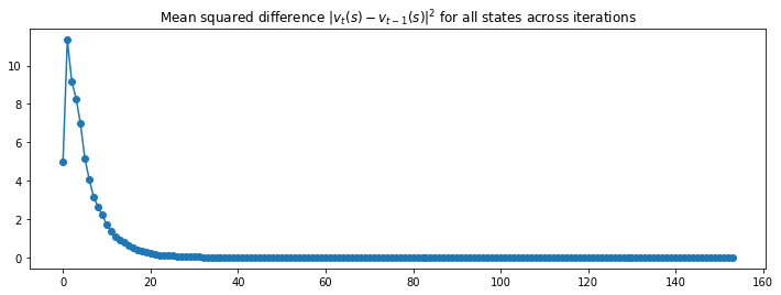
vstar, vs, diffs, QQ, RR = estimate_vstar(np.zeros_like(v), P, rewards)
Iteration 20, mean squared difference 0.2923686862066963
Iteration 40, mean squared difference 0.005394432111812179
Iteration 60, mean squared difference 7.973446958020696e-05
Iteration 80, mean squared difference 1.1785458612597435e-06
Iteration 100, mean squared difference 1.7419948416171354e-08
Iteration 120, mean squared difference 2.574822184066179e-10
Iteration 140, mean squared difference 3.805814524271806e-12
Final iteration 154, mean squared difference 1.5934112130695088e-13
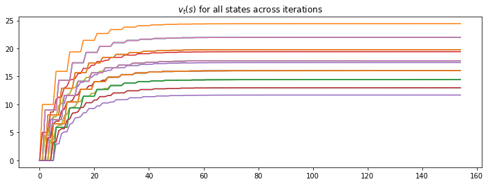
This converges very quickly to the optimal.
def plot_curves(vs, diffs):
    plt.figure(figsize=(12,4))
    plt.plot(vs);
    plt.title('$v_t(s)$ for all states across iterations')

    plt.figure(figsize=(12,4))
    plt.plot(diffs,'-o');
    plt.title('Mean squared difference $|v_t(s)-v_{t-1}(s)|^2$ for all states across iterations');
plot_curves(vs, diffs)
def plot_first_25(vs, states, th=8):
    vs_to_plot = vs[:25]
    vmin = np.min(vs_to_plot)
    vmax = np.max(vs_to_plot)
    plt.figure(figsize=(15,15))
    for i, vi in enumerate(vs_to_plot):
        plt.subplot(5,5, i+1)
        plt.imshow(make_grid(vi, [5,5]), vmin=vmin, vmax=vmax)
        plt.title('$v_{' + '%s}(s)$'%i)
        plt.axis('off');
        plot_grid(states, vi, -0.25, 0, th)
plot_first_25(vs, states)

def get_best_actions(QQ, RR, gamma=0.9):
    v_next_all = QQ + gamma*RR
    actions_best= []
    for vals in v_next_all:
        best_inds = np.where(vals==np.max(vals))
        actions_best.append(actions[best_inds])
    return actions_best
actions_best = get_best_actions(QQ, RR, gamma=0.9)
A note on the coordinate system
Again we can confirm that out results match the ones shown in the book. Note we are using the $ij$ matrix based axis rather than the usual $xy$ coordinate axis. That means when we move up in $xy$-coordinates, this corresponds to a down for the matrix since the row number $i$ decreases. Although left and right are equivalent, whilst moving left or right in $xy$ decreases or increases the $x$ coordinate, here the column $j$ decreases or increases. So for plotting our states and actions will be reversed. In order to facilitate comparision of the best actions to those shown in the book, we will reverse the action vectors and use down where the diagram in the book has up.
#Directions in xy world
right_xy = np.array([[1,0]])
left_xy = np.array([[-1,0]])
down_xy = np.array([[0,-1]])
up_xy = np.array([[0,1]])

#Directions in matrix world
right = up_xy
left = down_xy
down = right_xy
up = left_xy

right_up = np.concatenate([right, up])
up_left = np.concatenate([up, left])

actions_best_true = [right, actions, left, actions, left,
                     right_up, up, up_left, left, left,
                     right_up, up, up_left, up_left, up_left,
                     right_up, up, up_left, up_left, up_left,
                     right_up, up, up_left, up_left, up_left]
def actions_match(actions_true, actions):
    return (np.all(list(map(np.all, map(np.equal, actions_best, actions_best_true)))))
actions_match(actions_best_true, actions_best)
True
Confirm v_next is the same:
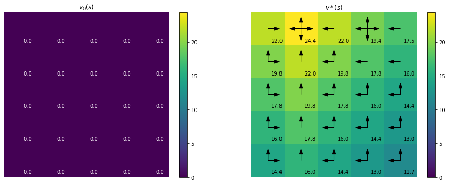
vstar_book = np.array([[22. , 24.4, 22. , 19.4, 17.5],
                        [19.8, 22. , 19.8, 17.8, 16. ],
                        [17.8, 19.8, 17.8, 16. , 14.4],
                        [16. , 17.8, 16. , 14.4, 13. ],
                        [14.4, 16. , 14.4, 13. , 11.7]])

values_match(vstar_book, vstar)
True
We will define a function to use below that will plot actions as arrows.
def plot_actions(ox,oy,length,actions,clr='k',**kwargs):
    for action in actions:
        plt.arrow(ox,oy,length*action[0], length*action[1],color=clr,**kwargs)
def plot_init_final(vs, states, actions_best):
    v_init_final = [vs[0], vs[-1]]
    vmin = np.min(v_init_final)
    vmax = np.max(v_init_final)
    plt.figure(figsize=(16,6))
    for i,(vi,title) in enumerate(zip(v_init_final, ['$v_0(s)$', '$v*(s)$'])):
        plt.subplot(1,2,i+1)
        plt.imshow(make_grid(vi,[5,5]),vmin=vmin,vmax=vmax)
        plt.title(title)
        plt.colorbar();

        if i == 1:
            for val, acts, (oy, ox) in zip(vi, actions_best, states):

                plot_actions(ox, oy, 0.2, acts[:,::-1], head_width=0.1)
        plot_grid(states, vi, 0.1, 0.4, 8)
        plt.axis('off');
plot_init_final(vs, states, actions_best)