Contents
Introduction: what is a Windrose?
A windrose, or a polar rose plot, is polar histogram that shows the distribution of wind speeds and directions over a period of time. It is a useful tool for visualising how wind speed and direction are typically distributed at a given location. The data is divided into direction intervals, and the frequency of wind speeds in each direction is represented by the radius of the bars. Typically the data is also binned into speed intervals and plotted as a set of stacked bars, where each bar represents a speed interval. The height of the bar is the frequency of wind speeds in that interval, and the radius of the bar is the sum of the frequencies of wind speeds in that interval.
In this tutorial we will learn:
- How to convert raw wind speed and direction data into a format suitable for plotting a windrose
- How to plot a windrose using Matplotlib and Plotly
- How to use Plotly and ipywidgets to create an interactive windrose
This blogpost can be found as a Colab notebook here.
Data preparation
The data used in this tutorial is available here. To following along download it and replace filepath below with the location at which you saved the data.
Data source
We have a dataframe containing wind speed and direction data measured at Coimbatore airport in India.
SPD- wind speed in m/sDIR- wind direction in degreesMM- month of the year between 1 and 12
Let us take a look at the first few rows of the data:
import calendar
import pandas as pd
import numpy as np
import matplotlib.pyplot as plt

# Modify to point to location where your data is saved
filepath = 'coimbatore-airport-2016.csv'
# Load data
df = pd.read_csv(filepath)

# Display the first few rows of the dataframe
df.head()
| NAME | HR_TIME | YYYY | MM | DD | HR | MN | TEMP | DEWP | SPD | DIR | |
|---|---|---|---|---|---|---|---|---|---|---|---|
| 0 | 433210-99999 | 2016010100 | 2016 | 1 | 1 | 0 | 0 | 65 | 62 | 5 | 360 |
| 1 | 433210-99999 | 2016010100 | 2016 | 1 | 1 | 0 | 0 | 64 | 63 | 5 | 360 |
| 2 | 433210-99999 | 2016010100 | 2016 | 1 | 1 | 0 | 30 | 64 | 63 | 3 | 360 |
| 3 | 433210-99999 | 2016010101 | 2016 | 1 | 1 | 1 | 0 | 64 | 63 | 3 | 360 |
| 4 | 433210-99999 | 2016010102 | 2016 | 1 | 1 | 2 | 30 | 66 | 63 | 3 | 20 |
Histogram Creation
First, we need to transform our raw wind data, which is a crucial step in constructing a windrose plot.
The windrose_histogram function partitions the raw wind speed and direction data into bins, counts the frequency of observations in each bin, and optionally normalizes these frequencies. The result is a 2D histogram, ideal for creating windrose plots.
def windrose_histogram(wspd, wdir, speed_bins=12, normed=False, norm_axis=None):
    """
    Compute a windrose histogram given wind speed and direction data.

    wspd: array of wind speeds
    wdir: array of wind directions
    speed_bins: Integer or Sequence, defines the bin edges for the wind speed (default is 12 equally spaced bins)
    normed: Boolean, optional, whether to normalize the histogram values. (default is False)
    norm_axis: Integer, optional, the axis along which the histograms are normalized (default is None)
    """

    # If speed_bins is an integer, we create linearly spaced bins from 0 to max speed
    if isinstance(speed_bins, int):
        speed_bins = np.linspace(0, wspd.max(), speed_bins)

    num_spd = len(speed_bins)
    num_angle = 16

    # Shift wind directions by 11.25 degrees (one sector) to ensure proper alignment
    wdir_shifted = (wdir + 11.25) % 360

    angle_bins = np.linspace(0, 360, num_angle + 1)

    # Generate a 2D histogram using the defined speeds bins and shifted wind directions
    hist, *_ = np.histogram2d(wspd, wdir_shifted, bins=(speed_bins, angle_bins))

    # Normalize if required
    if normed:
        hist /= hist.sum(axis=norm_axis, keepdims=True)
        hist *= 100

    return hist, angle_bins, speed_bins
This windrose_histogram function partitions the wind speed and direction data into bins, counts the frequency of observations in each bin, and optionally normalizes these frequencies. The result is a 2D histogram, ideal for creating windrose plots.
Data Transformation
Before diving into the intricacies of windrose plotting, we must first transform our raw wind data into a structured format that is more suitable for analysis. To achieve this, we’ll employ the following function:
DIRECTION_NAMES = ("N","NNE","NE","ENE"
                   ,"E","ESE","SE","SSE"
                   ,"S","SSW","SW","WSW"
                   ,"W","WNW","NW","NNW")

DIRECTION_ANGLES = np.arange(0, 2*np.pi, 2*np.pi/16)

# Mapping from direction name to angles in radians
NAME2ANGLE = dict(zip(
    DIRECTION_NAMES,
    DIRECTION_ANGLES
))

def make_wind_df(data_df, num_partitions, max_speed=None, normed=False, norm_axis=None, month=None):
    """
    This function transforms raw wind speed and direction data into a DataFrame for windrose plotting.

    data_df: Dataframe containing wind data
    num_partitions: Integer, number of partitions to divide the wind speed data
    max_speed: Float, optional, maximum wind speed to be included in the partitions
    normed: Boolean, optional, whether to normalize the frequency values
    norm_axis: Integer, optional, the axis along which the histograms are normalized
    """

    if month is not None:
        data_df = data_df[data_df.MM==month]

    wspd = data_df['SPD'].values
    wdir = data_df['DIR'].values

    # If max_speed is not specified, we use the maximum value in the 'wspd' data.
    # Otherwise, we include all speeds up to and including max_speed.
    # Additional partitions are created to handle outliers.
    if max_speed is None:
        speed_bins = np.linspace(0, wspd.max(), num_partitions + 1)
    else:
        speed_bins = np.append(np.linspace(0, max_speed, num_partitions + 1), np.inf)

    # windrose_histogram function is called to partition data based on the bins created.
    # Additional parameters control how the frequency values are normalised

    h, *_ = windrose_histogram(wspd, wdir, speed_bins, normed=normed, norm_axis=norm_axis)

    # A dataframe is formed containing the histogram data. Column names are for the directions
    wind_df = pd.DataFrame(data=h, columns=DIRECTION_NAMES)

    # speed_bin_names stores speed range strings to describe each interval
    # e.g. when speed_bins is [0, 3, 6], speed_bin_names is ['0-3', '3-6', '>6']
    speed_bin_names = []
    speed_bins_rounded = [round(i, 2) for i in speed_bins]
    for start, end in zip(speed_bins_rounded[:-1], speed_bins_rounded[1:]):
        speed_bin_names.append(f'{start:g}-{end:g}' if end < np.inf else f'>{start:g}')

    wind_df['strength'] = speed_bin_names

    # Reshapes data for plotting. Now, each row represents one sector of the windrose
    wind_df = wind_df.melt(id_vars=['strength'], var_name='direction', value_name='frequency')

    return wind_df
Here is what the dataframe looks like
make_wind_df(df, num_partitions=4).head(12)
| strength | direction | frequency | |
|---|---|---|---|
| 0 | 0-6.25 | N | 189.0 |
| 1 | 6.25-12.5 | N | 14.0 |
| 2 | 12.5-18.75 | N | 0.0 |
| 3 | 18.75-25 | N | 0.0 |
| 4 | 0-6.25 | NNE | 648.0 |
| 5 | 6.25-12.5 | NNE | 145.0 |
| 6 | 12.5-18.75 | NNE | 1.0 |
| 7 | 18.75-25 | NNE | 0.0 |
| 8 | 0-6.25 | NE | 815.0 |
| 9 | 6.25-12.5 | NE | 389.0 |
| 10 | 12.5-18.75 | NE | 15.0 |
| 11 | 18.75-25 | NE | 0.0 |
Making the plots
Using Matplotlib
Matplotlib is a versatile and comprehensive library in Python that allows for a wide variety of plotting types, such as scatter plots, bar charts, and line charts.
While Matplotlib does not have out-of-the-box capabilities to create a windrose, thanks to the library’s flexibility, we can make a plot which resembles a windrose using polar bar diagrams, where the height of the bars demonstrates the frequency of the wind speed, and the orientation of the bars represents the wind direction.
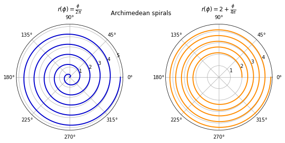
A polar plot is a diagram in which data points are represented in a polar coordinate system. In this system, a point’s location is determined by its distance from the centre (known as the radial coordinate $\rho$ or $r$) and by the angle from a reference direction (known as the angular coordinate $\phi$ or $\theta$).
Here is an example of a polar plot which shows an Archimedean spiral which can be represented by a linear polar equation
\[r(\phi) = a + b\phi\]We plot it with
\[a = 0, b = \frac{1}{2\pi} \quad \text{and} \quad a = 2, b = \frac{1}{4\pi}\]phi = np.linspace(0, 10*np.pi, 1001)
avals = [0, 2]
bvals = [1/(2*np.pi), 1/(4*np.pi)]
blabels = ['2\pi', '4\pi']
fig, axes = plt.subplots(1, 2, subplot_kw={'projection': 'polar'}, figsize=(10,4))
for clr, axis, a, b, bl in zip(['mediumblue', 'darkorange'], axes, avals, bvals, blabels):
axis.plot(phi, a + b*phi, linewidth=2, color=clr);
axis.set_title(f'$r(\phi) = {(str(a) + " + ") if a > 0 else ""}'
+"\\frac{\phi}{" + f'{bl}' +' }$' )
plt.suptitle(' Archimedean spirals');
In the context of windroses, we use polar plots for illustrating the wind direction (angular coordinate) and the wind speed (radial coordinate).
def matplotlib_windrose(data_df, num_partitions=4, max_speed=4, month=None):
    """
    Function to create a windrose plot using matplotlib.

    Args:
        data_df: Dataframe containing wind data
        num_partitions: number of partitions for wind strength
        max_speed: maximum wind speed to be considered while partitioning the wind strength
        month: (optional) a string representing the month, used in defining the DataFrame for plotting

    Returns:
        fig: a matplotlib Figure object containing the windrose plot
    """

    # calls the make_wind_df function to create a dataframe which
    # reshapes raw wind speed and direction data for windrose plotting
    wind_df2 = make_wind_df(data_df=data_df,
                        num_partitions=num_partitions,
                        max_speed=max_speed,
                        normed=True,
                        month=month)

    wind_df2['frequency'] = wind_df2['frequency']/ 100

    # modifies the dataframe by extracting start strength based on certain conditions in each strength value
    wind_df2 = wind_df2.assign(strength_start=[float(x.split('-')[0] if '-' in x else x[1:])
                                           for x in wind_df2.strength.values])

    # converts the mapped direction names to angles and sorts the dataframe according to the strength start
    wind_df2['angle'] = wind_df2.direction.map(NAME2ANGLE)
    wind_df2 = wind_df2.sort_values(by='strength_start')

    # The command below does three things sequentially:
    # 1. It sorts the dataframe 'wind_df2' in ascending order according to 'strength_start'.
    # 2. It groups this sorted dataframe by 'direction' so the each group contains the sorted values of 'strength_start' for the corresponding direction.
    # 3. It cumulatively sums the frequencies within each group (i.e., each unique wind direction) direction.
    # The cumulative frequency value for a given strength_start value is the sum of the frequencies of all the strength_start values that are less than or equal to the given strength_start value. The reason for doing this is to enable us to plot stacked bars in the windrose plot.
    wind_df2['cumulative_frequency'] = wind_df2.sort_values(by='strength_start').groupby('direction').frequency.cumsum()

    # Use black background
    with plt.style.context('dark_background'):
        # create a polar plot (windrose) with given figure size
        fig, axis = plt.subplots(figsize=(8, 8), ncols=1, subplot_kw=dict(projection="polar"))

        # adds a grid to the plot in white since background will be dark
        axis.grid(color='white')

        # extracts values from the 'strength_start' column of the dataframe
        strength_starts = wind_df2.strength_start.values

        # defines the colormap to be used for different strength partitions in the windrose
        colours = plt.cm.magma_r(
            np.linspace(0, 1,  wind_df2.strength.nunique())
        )

        # groups the dataframe by 'strength'
        strength_splits = wind_df2.groupby('strength')

        # plots a bar chart for each unique strength value in the windrose plot
        # in descending order of strength to make the bars appear stacked on top of each other
        # since the frequency values are cumulative, the bars are stacked on top of each other
        for clr, strength in list(zip(colours, wind_df2.strength.unique()))[::-1]:
            split = strength_splits.get_group(strength)
            # Note that the width is slightly less than 22.5 degrees (i.e., 360/16) so that the bars are slightly separated from each other which makes the plot look better
            # zorder=2 ensures grid does not appear on top of the bars
            axis.bar(split['angle'].values,
                     split['cumulative_frequency'].values,
                     color=clr,
                     label=strength,
                     width=np.deg2rad(19),
                     edgecolor='black',
                     linewidth=0.5,
                     zorder=2)

        # sets direction names as xticks in the windrose plot
        axis.set_xticks(DIRECTION_ANGLES)
        axis.set_xticklabels(DIRECTION_NAMES)


        # adds a legend to the plot
        handles, labels = axis.get_legend_handles_labels()
        axis.legend(
           handles[::-1],
           labels[::-1],
           loc='upper left',
           bbox_to_anchor=(1.1, 1.1)
        );

        # sets the zero location of the theta axis to North
        axis.set_theta_zero_location('N')

        # sets the direction of the theta axis to clockwise (-1)
        axis.set_theta_direction(-1)

        axis.set_title('Wind rose ({})'.format(
                               calendar.month_name[month] if month in range(1, 13) else 'Annual'
                           ))

        axis.set_rlabel_position(135)
        yticks = axis.get_yticks()
        ytick_labels = [('{:.2f}'.format(round(i * 100, 2))[:-1]).rstrip('0').rstrip('.') + '%' for i in yticks]
        axis.set_yticks( yticks)
        axis.set_yticklabels(ytick_labels)

    # returns the figure containing the windrose plot
    return fig
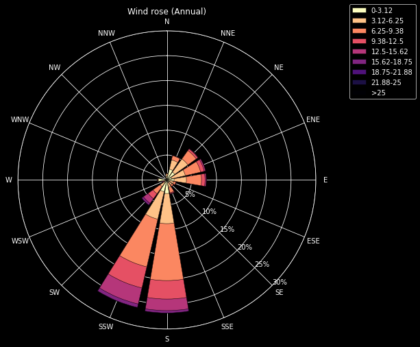
To use the matplotlib_windrose function, you pass in the wind dataframe plus additional arguments to vary the appearance of the plot. Below we shall see how to add interactivity so that we can vary these parameters and update the plot each time.
matplotlib_windrose(df, num_partitions=8, max_speed=25);
Implementing with Plotly
For an alternative approach, we turn to Plotly, another Python library known for its advanced plotting capabilities. We can leverage Plotly Express to achieve a straightforward realisation of a windrose plot.
The plotly_windrose function operates similarly to the make_wind_df function but utilizing Plotly’s ‘px.bar_polar’ to create the windrose plot, enhancing the plot with interactive capabilities.
import plotly.express as px

def plotly_windrose(data_df, num_partitions=4, max_speed=4, month=None):
    """
    Function to generate a windrose plot using Plotly.

    Args:
        data_df: Dataframe containing wind data
        num_partitions: number of partitions for wind strength
        max_speed: maximum wind speed to be considered while partitioning the wind strength
        month: (optional) a string representing the month, used in defining the DataFrame for plotting

    Returns:
        plot: a Plotly Figure object containing the windrose plot
    """

    # Convert raw data into a windrose-friendly format
    wind_df = make_wind_df(data_df=data_df,
                       num_partitions=num_partitions,
                       max_speed=max_speed,
                       normed=True,
                       month=month
                     )
    # Normalize frequency to a percentage
    wind_df['frequency'] = wind_df['frequency'] / 100


    # Sort strength bins in order
    strengths = sorted(wind_df.strength.unique(), key=lambda x:float(x.split('-')[0] if '-' in x else x[1:]))

    # defines the colormap to be used for different strength partitions in the windrose
    colours =px.colors.sample_colorscale(px.colors.get_colorscale('Magma_r'), len(strengths))

    colour_dict = dict(zip(strengths, colours))

    # Create a polar bar plot with the specified properties
    fig = px.bar_polar(wind_df, r="frequency", theta="direction",
                       color="strength",
                       color_discrete_map=colour_dict,
                       template="plotly_dark",
                       title='Wind rose ({})'.format(
                           calendar.month_name[month] if month in range(1, 13) else 'Annual'
                       )
                   )
    # Update the polar plot parameters to enhance readability and esthetics
    fig.update_polars(
        radialaxis_angle = -45, # To rotate the radial axis
        radialaxis_tickangle=-45, # To rotate the tick labels on radial axis
        radialaxis_tickformat=',.0%', # To change the tick labels to percentages
        radialaxis_tickfont_color='white', # To change tick labels to white for better readability,
    )

    # Make figure square
    fig.update_layout(
        autosize=False, # To prevent automatic adjustment of figure size
        width=500, # To set figure width to 500 pixels
        height=500, # To set figure height to 500 pixels
    )

    return fig
Creating a plot with plotly_windrose we can see that it looks very similar to the previous plot but with Plotly’s interactive features.
plotly_windrose(df, num_partitions=8, max_speed=25)
Interactive plotting using Matplotlib and Jupyter Widgets
The plots so far have shown windroses using the entire dataset. However, wind patterns can vary significantly depending on the time of year. We can use Jupyter widgets to create an interactive windrose that allows us to select the month of the year to plot.
In addition, we can also choose the number of partitions and the maximum wind speed to be included in the plot. These settings will give use greater control over the appearance of the windrose.
Widgets are interactive controls for python within Jupyter notebooks, allowing you to dynamically change variables and view the changes in output.
To create an interactive widget, we can use the interact function of the ipywidgets library. The interact function automatically creates user interface (UI) controls for function arguments, and then calls the function with those arguments when you manipulate the controls interactively.
In addition our widget will let us choose which of the two plotting libraries we want to use, Matplotlib or Plotly.
from ipywidgets import interact, fixed, IntSlider, Dropdown, Layout, Output
month_dict = {('Annual' if i == 0 else calendar.month_name[i]):i for
i in range(13)}
def interactive_windrose(num_partitions, max_speed, month, method):
fn = {'Plotly': plotly_windrose, 'Matplotlib': matplotlib_windrose}[method]
f = fn(df, num_partitions=num_partitions,
max_speed=max_speed, month=month if month > 0 else None)
if method == 'Plotly':
f.show()
interact(interactive_windrose,
num_partitions=IntSlider(value=5, min=2, max=33, description='No. partitions',
layout=Layout(width='400px'),
style=dict(description_width='initial')),
max_speed=IntSlider(value=17, min=2, max=33, description='Max wind speed (m/s)',
layout=Layout(width='450px'),
style=dict(description_width='initial')),
month=Dropdown(options=month_dict, value=3, description='Month',
layout=Layout(margin="0px 0px 10px 0px"),
style=dict(description_width='initial')),
method=Dropdown(options=['Plotly', 'Matplotlib'], value='Plotly', description='Method',
layout=Layout(margin="0px 0px 25px 0px"),
style=dict(description_width='initial'))
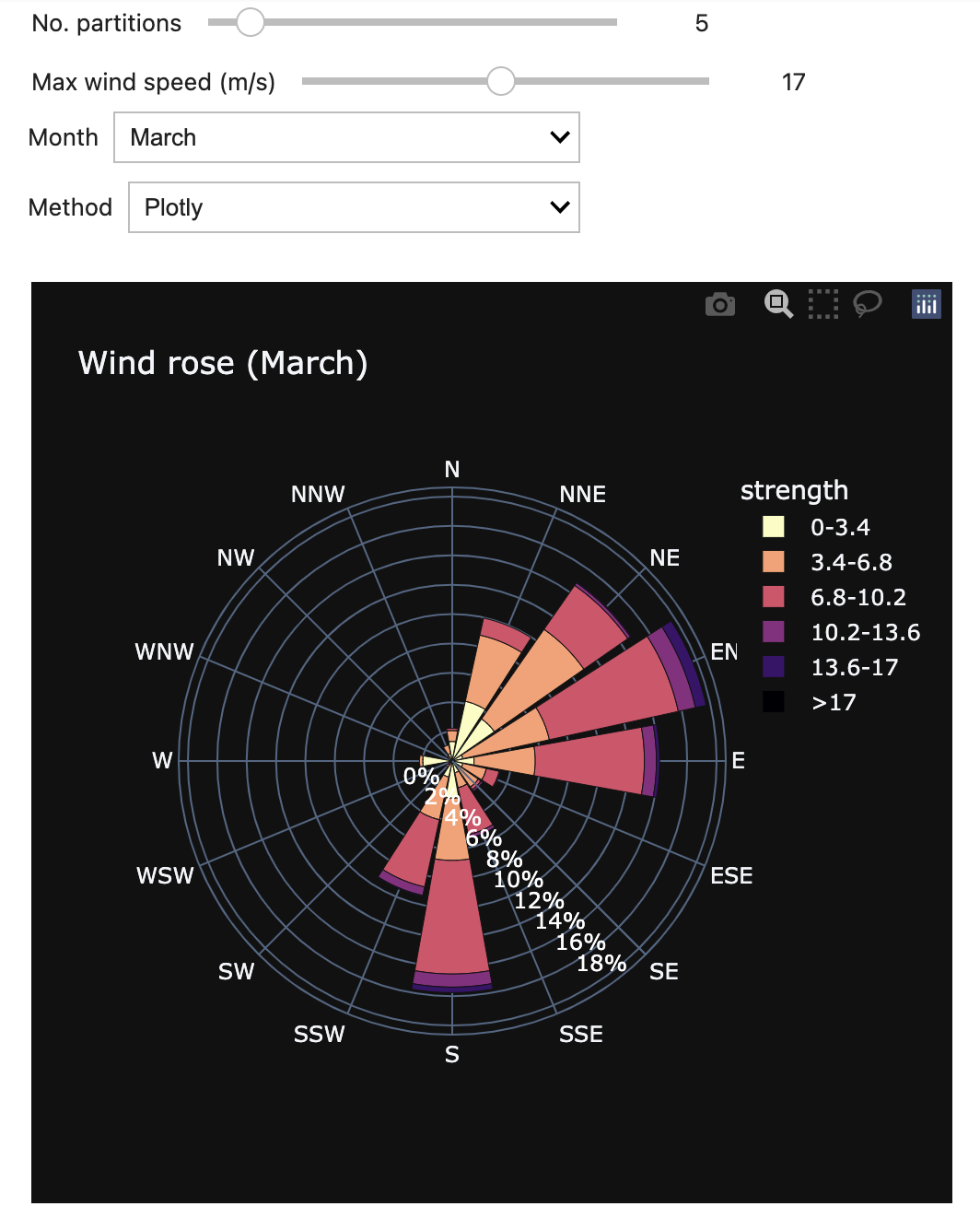
);
This is what the widget looks like. You can try it out for yourself in the Colab for this blog.
Conclusion
In this tutorial, we have walked through the process of plotting a windrose, a polar plot which shows the distribution of wind speeds and directions over time. We covered the essential knowledge behind windroses, walked through some methods of data preparation, and learned to generate windroses using two notable Python libraries - Matplotlib and Plotly. Furthermore, we touched upon how to add interactivity to our windrose plots with Jupyter widgets, enhancing their usefulnesses. The techniques covered in this tutorial can be leveraged in meteorology, climate studies, aviation and other fields requiring wind data analysis and visualisation.