
Contents
- Introduction
- Creating a Single Qubit Quantum Gate - X gate
- Creating a Diagram
- Saving the Diagram Figure
- Single Gate Example: Hadamard
- Two Qubit Gate Example: CNOT
- Creating Custom Gates
- Creating Circuit Diagrams
- Conclusion
Introduction
Quantum computing is a rapidly growing field that leverages the principles of quantum mechanics to process information. One of the pillars of quantum computing is the quantum circuit, a model for quantum computation in which a computation is represented by a sequence of quantum gates. In this blog we will learn how to create quantum gate and quantum circuit diagrams in Python using the SymPy library.
SymPy is a Python library for symbolic mathematics. It includes a module for quantum computing called sympy.physics.quantum which we will use to create quantum gates and circuits and to generate their diagrams. We will start from simple single qubit gates to more complex two qubit gates and finally learn to create custom gates and quantum circuits.
This tutorial assumes that you have basic knowledge of quantum computing and quantum gates. I am planning on writing a blog on quantum gates soon, but until then I recommend this Wikipedia article as a good reference for quantum gates.
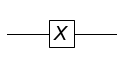
Creating a Single Qubit Quantum Gate - X gate
Let’s start by creating an X gate, also known as a NOT gate. The X gate acts on a single qubit. It is represented by the following matrix:
\[X = \begin{bmatrix}0 & 1 \\ 1 & 0\end{bmatrix}\]SymPy has a number of commonly used quantum gates already defined. To instantiate a gate, you need to specify the qubit or qubits it acts.
Key qubit numbering conventions in SymPy:
- Qubits are zero-indexed, so the first qubit is 0, the second is 1, and so on.
- Qubits are numbered starting from the bottom so the wire at the bottom of the diagram stands for qubit 0, the next one above is 1, and so on.
Let’s now create an X gate acting on the first qubit.
from sympy.physics.quantum.gate import X

gate = X(0)
Creating a Diagram
In order to plot our quantum gate, we’ll use the plot function from the circuitplot module. The plot function takes two arguments, the gate and the number of qubits in the circuit. Let’s plot the X gate we created above.
import sympy.physics.quantum.circuitplot as plot
plot.circuit_plot(gate, 1);
Saving the Diagram Figure
Saving the generated quantum circuit figure is a straightforward process. You can use the savefig function from the matplotlib package to save the figure. Let’s save the figure we generated above.
import matplotlib.pyplot as plt
plt.savefig("X_gate.png");
<Figure size 432x288 with 0 Axes>
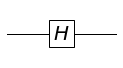
Single Gate Example: Hadamard
The Hadamard gate or $H$ gate is a one-qubit gate which performs a Hadamard transform on the given qubit.
It is represented by the following matrix:
The steps to create a Hadamard gate are the same as the X gate. Let’s create a Hadamard gate acting on the first qubit and plot it.
from sympy.physics.quantum.gate import H
H_gate = H(0)
plot.circuit_plot(H_gate, 1);
Two Qubit Gate Example: CNOT
Controlled NOT gate, or CNOT, is a two-qubit gate which takes two inputs, a control and a target qubit and applies a NOT to the target only when the control is $\left\vert 1\right>$. We use the notation CNOTxy to denote a gate where the qubit with index $x$ is the control and qubit with index $y$ is the target.
The matrix representation of CNOT21 i.e. CNOT with the second qubit as the control and the first qubit as the target is:
\[\begin{bmatrix} 1 & 0 & 0 & 0 \\ 0 & 1 & 0 & 0 \\ 0 & 0 & 0 & 1 \\ 0 & 0 & 1 & 0 \end{bmatrix}\]I should note that you may find other sources that represent the CNOT gate with the target qubit as the first qubit and the control qubit as the second qubit in which case the above would be the matrix representation of CNOT12. However I have tried to use notation that is consistent the way the gates are instantiated in SymPy.
The CNOT class in SymPy takes two arguments, the control qubit index and the target qubit index in that order. Let us first construct and plot a CNOT21 gate.
from sympy.physics.quantum.gate import CNOT
CNOT_21 = CNOT(1, 0) # Note the zero based indexing so that 2->1, 1->0
plot.circuit_plot(CNOT_21, 2);
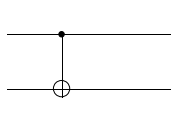
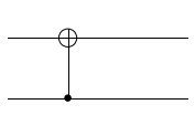
Note that in the diagram the the qubits are numbered from top to bottom. The topmost wire corresponds the first index, the second wire to the second index and so on. Now let’s plot a CNOT12 gate, where the control and the target are reversed.
CNOT_12 = CNOT(0, 1)
plot.circuit_plot(CNOT_12, 2);
Creating Custom Gates
X Gate represented as a NOT gate
If you look at the matrix for $X$ you can see that it flips qubits turning $\left\vert 0\right>$ to $\left\vert 1\right>$ and $\left\vert 1\right>$ to $\left\vert 0\right>$. (Recall that the vector representations of the qubits are $\left\vert 0\right> = [1, 0]^T$ and $\left\vert 1\right> = [0, 1]^T$).
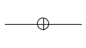
The gate is often represented using the symbol $\oplus$ that’s used in the CNOT gate. X has a built in function plot_gate_plus that can plot the gate using this symbol but it is not used by circuit_plot. Let us subclass X to create XNOT, where we redefine the plot_gate function as an alias for the plot_gate_plus function, maintaining identical functionality otherwise so that now circuit_plot will plot X using the desired symbol.
class XNOT(X):
    plot_gate = X.plot_gate_plus

plot.circuit_plot(XNOT(0), 1);
Rotation Gate
You can use the UGate class to create a custom quantum gate. As an example, we’ll create a rotation gate. The rotation of a qubit by an angle $\theta$ around the Y-axis of the Bloch sphere is represented by the following matrix:
Here, $R_Y(\theta)$ represents the Y-axis rotation gate, $I$ is the identity matrix, and $Y$ is the Pauli $Y$ matrix, which is defined as:
\[Y = \begin{bmatrix} 0 & -i \\ i & 0 \end{bmatrix}\]To create a Y rotation gate from the UGate class, you need to instantiate the class with the following arguments:
- The qubit the gate acts on
- The matrix representation of the gate
Let us write a simple function to create a Y rotation gate.
from sympy.physics.quantum.gate import UGate
import sympy as sy

def R_Y(qubit, theta):
    Y_sy = sy.Matrix([[0, -sy.I], [sy.I, 0]])
    gate = UGate(qubit, sy.eye(2)*sy.cos(theta/2) - sy.I * Y_sy * sy.sin(theta/2))
    return gate
Let us now define an $R_Y\left(\frac{\pi}{4}\right)$ gate.
R_Y_piby4 = R_Y(0, sy.pi/4)
If you now try to plot the gate, this is what it looks like:
plot.circuit_plot(R_Y_piby4, 1);
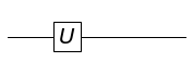
As you can see this is labeled as a generic $U$ gate. To customize the label, you can modify the gate_name_latex attribute of the gate. Let’s update the function accordingly.
def R_Y(qubit, theta):
    Y_sy = sy.Matrix([[0, -sy.I], [sy.I, 0]])
    gate = UGate(qubit, sy.eye(2)*sy.cos(theta/2) - sy.I * Y_sy * sy.sin(theta/2))
    name = f'R_Y\\left({sy.latex(theta)}\\right)'
    gate.gate_name_latex = name
    gate.gate_name = name
    return gate
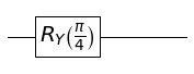
Now, if you create and plot the gate again, you’ll see it is correctly labeled as $R_Y\left(\frac{\pi}{4}\right)$.
R_Y_piby4 = R_Y(0, sy.pi/4)
plot.circuit_plot(R_Y_piby4, 1);
Toffoli Gate
We can also construct custom multi-qubit gates. As an example, let’s create a Toffoli gate which takes three inputs, two of which are controls whilst the other is the target. The Toffoli gate applies a NOT to target only when both controls are $\left\vert 1\right>$. It is effectively a controlled-CNOT gate.
The matrix representation of the Toffoli gate is:
\[\begin{bmatrix} 1 & 0 & 0 & 0 & 0 & 0 & 0 & 0 \\ 0 & 1 & 0 & 0 & 0 & 0 & 0 & 0 \\ 0 & 0 & 1 & 0 & 0 & 0 & 0 & 0 \\ 0 & 0 & 0 & 1 & 0 & 0 & 0 & 0 \\ 0 & 0 & 0 & 0 & 1 & 0 & 0 & 0 \\ 0 & 0 & 0 & 0 & 0 & 1 & 0 & 0 \\ 0 & 0 & 0 & 0 & 0 & 0 & 0 & 1 \\ 0 & 0 & 0 & 0 & 0 & 0 & 1 & 0 \end{bmatrix}\]To construct the Toffoli we can use the CGate class. The CGate class takes two arguments:
- A list of control qubits
- The gate to be applied to the target qubit
Since the Toffoli gate can be represented as controlled CNOT gate, we can create a Toffoli gate as follows:
from sympy.physics.quantum.gate import CGate
control_qubit1 = 2
control_qubit2 = 1
target_qubit = 0

toffoli_1 = CGate([control_qubit1], CNOT(control_qubit2, target_qubit))
plot.circuit_plot(toffoli_1, 3);

You can also regard the Toffoli gate as a doubly-controlled NOT gate where the first two qubits are controls and the third qubit is the target. In this case, we can create a Toffoli gate (using XNOT to ensure the NOT symbol is used in the plot) as follows:
toffoli_2 = CGate([control_qubit1, control_qubit2], XNOT(target_qubit))
plot.circuit_plot(toffoli_2, 3);
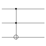
As you can see, both the representations are equivalent and lead to identical gate diagrams.
Creating Circuit Diagrams
A sequence of quantum gates gives rise to a quantum circuit. You can construct a quantum circuit in SymPy by multiplying gates together in the order in which you want them to be applied in the circuit
Single Qubit Circuit - Hadamard in terms of $X$ and rotation gates
A simple quantum circuit uses $X$ and rotation gates to create a $H$ gate. It is straightforward to show that
\[H = R_Y\left(-\frac{\pi}{4}\right)X R_Y\left(\frac{\pi}{4}\right)\]Let’s create and plot the circuit in SymPy
circuit = R_Y(0, -sy.pi/4) * X(0) * R_Y(0, sy.pi/4)
plot.circuit_plot(circuit, 1);
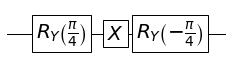
Note that since the gates in the circuit are applied from left to right, the order of the gates in the circuit is the reverse of the order in which they are multiplied to form $H$. To confirm that the circuit is indeed equivalent to the $H$ gate, we can use the represent function from the represent module to get the matrix representation of the circuit.
from sympy.physics.quantum.represent import represent
represent(circuit, nqubits=1).simplify()
$\displaystyle \left[\begin{matrix}\frac{\sqrt{2}}{2} & \frac{\sqrt{2}}{2}\\frac{\sqrt{2}}{2} & - \frac{\sqrt{2}}{2}\end{matrix}\right]$
which is indeed the matrix representation of the Hadamard gate.
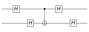
Multi-Qubit Circuit - using Hadamard gates to swap CNOT control and target
Now we will implement a more complex circuit involving 2 qubits. The CNOT has a certain property that if you apply a Hadamard gate to both qubits at the input as well as the output, you get a CNOT gate with the control and target qubits swapped.
Let’s see how this comes about. First, a Hadamard gate applied in parallel to both qubits gives rise to the following matrix
\[H\otimes H = \frac{1}{2}\begin{bmatrix} 1 & 1 & 1 & 1 \\ 1 & -1 & 1 & -1 \\ 1 & 1 & -1 & -1 \\ 1 & -1 & -1 & 1 \end{bmatrix}\]The CNOT12 gate has the following matrix
\[CNOT_{12} = \begin{bmatrix} 1 & 0 & 0 & 0 \\ 0 & 0 & 0 & 1 \\ 0 & 0 & 1 & 0 \\ 0 & 1 & 0 & 0 \end{bmatrix}\]Use these two matrices it is straightforward to show that
\[H\otimes H\cdot CNOT_{21}\cdot H\otimes H = CNOT_{12}\]Let us plot the circuit
circuit = H(0) * H(1) * CNOT_21 * H(0) * H(1)
plot.circuit_plot(circuit, 2);
We can also get the matrix representation of the circuit to confirm that it is indeed a CNOT12 gate.
matrix = represent(circuit, nqubits=2)
from IPython.display import Markdown
## Needed to make the matrix display correctly in the markdown document
Markdown(f'$${sy.latex(matrix)}$$')
Conclusion
In this blog, we learned how to create quantum gate and quantum circuit diagrams using Python’s SymPy library. We started by creating single qubit gates like the X gate and Hadamard gate. We then moved on to creating multi-qubit gates like the CNOT gate and Toffoli gate. Finally, we learned how to create custom gates and quantum circuits.
This only scratches the surface of SymPy’s quantum computing capabilities and of quantum computing in general. If you want to learn more about quantum computing, I recommend checking out the MIT Open Learning courses on Quantum Information Science (courses 8.370 and 8.371). For more about SymPy’s quantum computing capabilities, check out the SymPy documentation.